ALTRO Setup for STAR TPC

Jeff Landgraf

I. Introduction

The goal is to figure out the best running modes for the ALTRO under the DAQ 1000 project, and to get a good idea of the performance of the PASA/ALTRO shaping, pedestal subtraction, tail subtraction and zero suppression functionality. To this end, I first examined the raw output of the TPC with real events. I then discuss my recommendations for the ALTRO operating modes. Because the DAQ1000 project will replace the shaping circuitry, I then compiled a model for the analog readout of the STAR TPC using the PASA. Finally, I use both the STAR data and the TPC simulation to study the response of the ALTRO tail cancellation and zero suppression.

II. Characterization of STAR Data

Data Set

For almost all studies I used one sector (sector 1), of one event (event #8, run 6049037) which satisfied the min-bias trigger. This event was written out with no pedestal subtraction or zero suppression, but with the standard 10-8 bit gain conversion. I used the pedestals calculated during the previous pedestal run (#6049049).

A simple display of hits, clearly shows real tracks in this data. Here I show pedestal subtracted adc values>20 in padrow/pad/tb coordinates.

ADC Spectrum

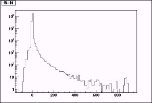
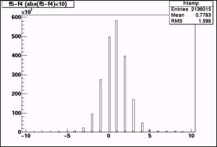
Here is the pedestal subtracted ADC spectrum. At low values, the noise looks like a reasonable gaussian with RMS = 1.6 ADC counts. The mean is .77 ADC values. This may represent a slight pedestal drift. It might also represent a small fraction of real hits, although the RMS is calculated with the ADC<10 cut.

ADC Saturation

The pedestal subtracted ADC distribution shows a peak at ~900ADC counts. This is due to saturation of the dynamic range. The width of the peak is due to differing pedstal values for the saturated pads. ~.1 % (9 sequences of ~10,000) saturate in the TPC data. The saturation value is 1003 adc counts (8-bit value is 253 instead of 255)

Representative Cluster Shapes

Here are three views of the hit with the biggest ADC value hits in the inner sector:

Sector 1: row 8: pad 121

You can see quite clearly the ADC saturation for this hit. Also note that there is a significant undershoot where the ADC value drops below zero in time-bins following the hit. Finally note that there are actually two well separated hits, the second arriving in the undershoot region. Here I plot the ADC vs time for two pads involved in this hit. The first pad is saturated, and it includes a contribution from the second hit. The second pad is away from the second hit and never saturates.

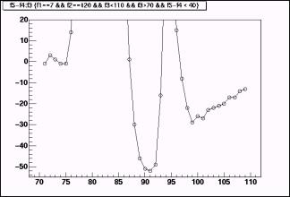
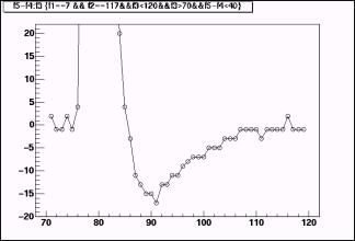
For pad 117 (The well separated peak), the integral of the charge in the positive region is 2371 adc counts. In the negative region it is 184 adc counts. So we find that the integral of the undershoot is 7.7% of the peak. The ratio of the maximum peak undershoot to the peak height is 2.2%.

Here is a similar cluster for the outer sector (row 40: pad 35)

In this case, the hit seems to be the accumulation of at least three and maybe six hits. The ratio of the undershoot height to peak height is consistent with, but slightly larger than the well separated peak ~2.9%. This can be understood because the peak is sharper than the undershoot, so the staggering of the hits doesn’t add as much to the peak as to the undershoot.

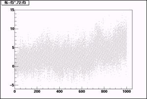
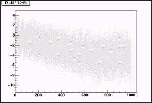
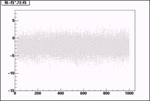
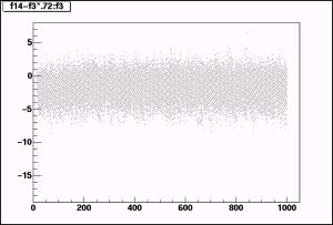
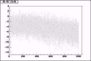
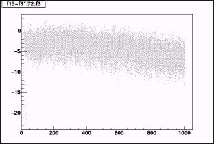
Undershoot parameterization

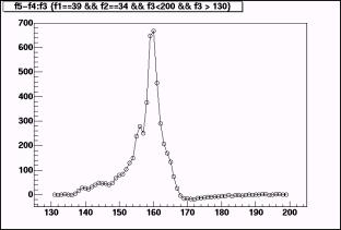
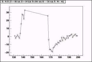
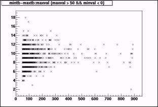
To study the shape of the undershoot in more detail, I looked at the ratio of the valley to the peak. To do this, I required a local minimum to follow a local maximum by less than 20 time buckets. I then cut out local maximum that were greater than 0, to get rid of noise &/or overlapping hits. Here is the undershoot vs the max value. I also plot the time between the peak and the maximum undershoot. This is ~9 time bins independent of the size of the peak.

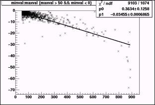
The large drop near 900 is an effect of the 10-bit saturation of large sequences. The peak saturates, but not the undershoot.

Because the size of the undershoot scales well with the size of the hit, and because the time to reach the minimum value is constant with respect to the size of the hit, I conclude that the shape of the undershoot is reasonably independent of the pulse size.

Another Representative Hit

I thought that this hit is somewhat interesting. The following plots show the ADC values vs pad and time for pad row 32 and 33. They show what I original believed to be a noisy fee card. The reason for this is that the island of charge roughly corresponds to a FEE 59 which spans pads 96-111 on pad rows 32 & 33.

The final plot is a real space plot of the hits>10 in row/pad/tb coordinates. From this plot it is clear that the “noise” is really a looping electron. The radius of the helix is small enough that the standard STAR tracking algorithms will not track this well. However, because you can easily get the momentum of the electron from the radius of the helix, and because the clusters sizes are small, this and similar clusters might be an avenue for a tracking independent study of dE/dx.

III. ALTRO Operating modes for DAQ 1000

The ALTRO breaks the signal processing up into four stages independent stages which are applied in series.

1. Base-Line Correction 1

2. Tail Subtraction

3. Base-Line Correction 2

4. Zero Suppression

Base-Line Correction 1

Base-Line Correction 1 has two components. The ALTRO continuously performs adc conversion even when there is no active event, so the first component is an “out of window” pedestal subtraction which takes effect when there is no active triggered event. The algorithm they use is to subtract a pedestal value called vpd. This parameter is an average of the current adc value with the previous adc value. It follows the input signal with a time constant of about 1 clock cycle. I have no way to study the usefulness of this filter currently, as STAR has no data whatsoever during the period when the gated grid is closed. Because we have large transients when the gated grid opens, I expect that this feature will be useless and turned off.

The second component of Base-Line Correction 1 is “in window” pedestal subtraction which takes effect during the event. There are numerous modes. The subtraction modes allow subtraction of constant adc values (either a user supplied fixed value fpd, or the out of window value vpd), time dependent user supplied pedestals, or gain correction. The pedestals may be set by pad. The altro uses the same memory to store the gain correction lookup table as it does to store the time-dependent pedestal values, so it is not possible to use gain correction and pedestal subtraction at the same time. The mode I expect to use is #1 (din – f(t)), although we might experiment with #6 (din – vpd – f(t)) once we have a working system. Mode #1 maps precisely to the same pedestal subtraction method used in STAR. One difference between STAR’s current electronics and the new system is that in the current system the exponential tail subtraction is done by the SAS chip which is applied before pedestal subtraction. In the new system, pedestal subtraction is applied first.

Note that for Base-line Correction 1, the “out of window” procedure uses an online procedure to choose a value, vpd. Once the event is triggered, vpd, is simply a constant number. It is not modified again during the readout of the event. There is no other adaptive procedure in Base-Line Correction 1.

Tail Subtraction

Tail subtraction is performed by a digital filter with 6 independent parameters. This filter is described in detail later in this document. The filter will likely be disabled for pedestal and pulser runs, but will be used in data runs.

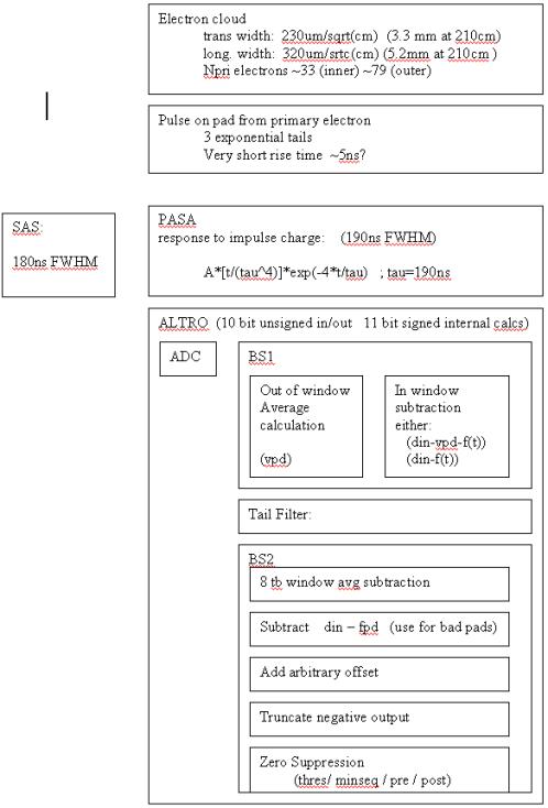
Figure 1. Altro signal flow

Base-Line Correction 2

Base-Line Correction 2 is an “in window” moving average pedestal subtraction (MAU) which is applied after the tail subtraction. The pedestal is defined as the average of the previous 7 samples. In order to remove actual data hits from the averages there are two thresholds which define a window. If the adc value is outside of the range thr_hi + curr_adc < x < curr_adc – thr_low, then the sample is excluded from the running average. Additionally, one can expand the exclusion region by fixed a fixed number of presamples and postsamples.

The current STAR TPC pedestal subtraction works quite well, However, additional effects such as small pedestal drifts, and incomplete tail subtraction might be corrected by the moving average filter. When we have a working system we can check this in detail. In the worst case, it will have no beneficial effect and can be turned off.

After the MAU filter has been applied, one has the option to add a constant offset to the data. After this offset is applied, negative adcs are truncated to zero.

Zero Suppression

The current STAR zero suppression is based on the DAQ ASIC, which uses four parameters: seq_hi, seq_lo, thr_hi, and thr_lo. The ASIC delineates sequences for which the ADC value exceeds thr_lo for more than seq_lo timebins and also exceeds thr_hi for more than seq_hi timebins.

The ALTRO zero suppression is less complex. It uses two parameters: thr, and seq. It delineates sequences for which the ADC values exceeds thr for more than seq timebins. However, the ALTRO also uses two more parameters, pre and post, to expand the sequence to include timebins before and after the threshold is met.

Finally, on the ALTRO, sequences are merged together if there is a gap of two or less timebins between them.

IV. The Model for the TPC Simulation

The basic idea for my TPC modeling is that the signal that is digitized by the ALTRO comes from four main effects:

1. The shape of the drifting electron cloud

2. The physical response on the TPC pad to a delta function pulse

3. The response of the PASA shaping chip (or the SAS in the current STAR TPC)

4. The integration and ADC conversion of the charge in timebins.

I model the TPC response by constructing models for first three signals and convoluting them. I normalized all of these shapes to unity. I used the study of TPC raw data to see the charge spectrum in units of ADC values. All Q response functions are presented in units of ADC.

Electron Cloud

The electron cloud shape is assumed to be gaussian. Sigma is obtained by , where x is the drift distance. For completeness, the dispersion in the transverse direction is , (ref 4) although this is not used in any of the following analysis. I always assume a perpendicular crossing angle, however, reasonable crossing angles can be approximated by simply increasing the effective drift distance.

Physical Response of the TPC

The TPC pad response to a delta function pulse is modeled as the sum of three exponentials. For P10 gas, (ref 4) gives

This obviously explodes at low t. There is a measured plot in the same reference that shows a very rapid initial response with a peak at ~2-3ns. I fudged this initial response by multiplying the above response by

The normalization was calculated numerically.

PASA Shaping response

The PASA response was taken from (ref 3)

Where again the normalization was calculated numerically.

Numerical Methods

To perform the convolutions I used the Fourier transform package FFTW from MIT. One has to be quite careful performing multiple convolutions using this package because the input is assumed to have the range –x to x, whereas the output has the range 0 to 2x. In order to get the convolutions right, the results must be shifted appropriately using the property that the results are periodic in the sample length. I used vastly expanded integration ranges (-8000 – 8000 ns) to avoid aliasing effects in the convolutions. I used 100,000 sampled points to avoid artifacts arising from the discreet sampling rate.

Here I show the results of this model.

The final pulse width is dominated by the PASA shaping, although a very slight dependence on the drift distance is also seen. The tail is completely dominated by the exponential decay functions.

Calculation of the ADC values

To get the digitized ADC values for each time-bin, I integrated the pad response. This gives slightly different results than taking the value of the response at the center of the time-bin. The effect is reasonably small. For small clusters, it makes effectively no difference because of quantization, but for large clusters the effect can certainly be noticed. Although it only matters in the peak where the adc changes rapidly. (Plots are for 10cm drift. Black line is the TPC response. Circles are ADCs obtained by value. Crosses are by integral. The red lines incorporate the tail subtraction to be discussed later.)

Comparison to measured data

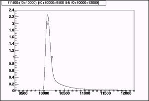
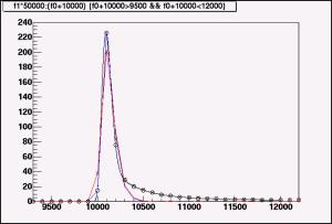
As a sanity check I compared the simulation to real data. The following plots compare simulated 100cm drift for calculated cluster using PASA shaping & ALTRO tail suppression to real data. The real data has a drift distance of ~50cm. The calculated pulse was scaled and shifted to best match the real data and is shown for two different tail suppression settings (to be discussed). The real data has a slightly wider pulse despite having a shorter drift distance. This might be due to the difference between the SAS and the PASA, or it might be due to a non-zero crossing angle for this track. The STAR tail suppression undershoot is larger than the optimal ALTRO suppression.

V. ALTRO Tail Cancellation

Analytic Calculation of the Tail Cancellation parameters.

The ALTRO tail cancellation circuit is a digital filter that is described in (ref 1) and (ref 6). The description of the filter is given in the “Z domain”. This is effectively the discreet version of the Laplace transform defined by:

Where T is the time step. This transformation is useful in filters because it has the same behavior as the fourier and laplace transforms with respect to convolutions. The convolution of two functions in the z-domain is the product. If the filter transfer function is given in the z-domain, all you need to do is multiply it by the z-domain version of the input signal to get the response. If you want the final output of the filter, you would then rewrite the result in the time domain.

The z-domain representation of three exponentials is just:

The z-domain representation of the ALTRO tail cancellation filter, unfortunately, is inconsistent between (ref 6) and the Altro User Manual (ref 1). Even worse, the version in the ALTRO manual is wrong. The correct version of the transfer function is:

Because of the form of the transfer function, it is obvious that the order of the L and K constants do not matter. In order to calculate the appropriate values for the 6 constants, you need to try make the convolution, , independent of z (which will look like a delta function in t space).

So, by expanding I(z) its easy to see that the choice

Cancels the denominator of I(z) But the are harder to calculate. To get the K’s first expand the numerator of I(z) and multiply out the denominator of T(z)

Now, because all we are trying to do is to remove the z dependence, we are free to divide I(z) by a constant. Then to remove the z dependence, we demand that all of the z coefficients match. This, of course, is impossible, because of the term in the denominator of T(z). So, we simply minimize its coefficient. We obtain the following system of equations for the K’s

Numerically this is a simple procedure. The resulting values are:

L = .945, .675, .0556

K = .8568, .777, .0006

Notice, that it is impossible to remove completely, the z-dependence. One way to try would be to add a fourth exponential to the model of the Is(t). In this case, one would be able to completely cancel the K’s, but then there would be an extra factor in the denominator of Is(z). The choice made by here is to apply the hardest cut to minimize the tails, however, this leads to a pronounced undershoot in the data. It is not necessarily the best cut for physics. For the rest of this discussion I will call these cuts the “HARD” &/or “Calculated” tail cancellation cuts.

Setting Constants using Simulated Annealing

A second way to determine the filter constants is to use simulated annealing in the 6 parameter constant space, to find the constants that best minimize the tails using the ALTRO simulation. The algorithm works by taking random steps in the constant space proportional to a “temperature”. One accepts or rejects each step randomly by calculating an energy for the resulting state and using the Boltzman distribution. One then reduces the temperature gradually following an “annealing schedule” until an acceptable minimum is found.

To generate new values for the constants, I treated each independently:

Where T is the temperature and x a random variable between 0 and 1 and the sign of the step is also random. The energy is calculated by two RMS functions:

Here, Xin and Xout are the input and output of the tail filter, t is the time bin measured from the start of the pulse. Constants in the tail portion of the energy function emphasize the tail region, and were obtained by iteratively running the algorithm until obtaining good results.

The annealing schedule I used was to set t=1 and to subtract .00001 each cycle until reaching zero.

Results were the same for drift distances between 10cm and 200cm

L = .945, .675, .0556

K = .929, .553, .256

Tail Subtraction Results

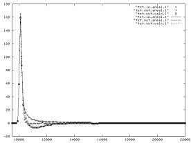
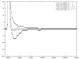
Here, obviously the simulated annealing is the best, the trouble with the calculation is the assumption about the fourth exponential. This could be made slower until there was no overshoot, in effect choosing the fourth exponential to match the trailing edge of the shapers pulse.

Here, I added many hits spaced at 10 rhic clocks from each other (1us). You can see that the errors for both the raw and for the “calculated” K’s accumulate for about 6us. This is a reflection of the time constant for the slowest exponential (2us) Again the simulated annealing Ks give almost perfect response

VI. Zero Suppression Studies

TPC ASIC values for the 2005 run are: thrlo = 1, thrhi = 4, seqlo = 2, seqhi = 0. My goal here is to

determine how compatible the ASIC sequence definition is with the zero suppression algorithm of the ALTRO and to figure out the best settings for the ALTRO.

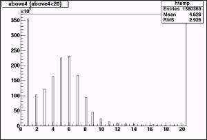
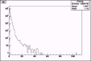
I start by characterizing the hits from a normal min-bias run using the current ASIC parameters. The first plot is the distribution of #of hits above the high threshold in star data. There are many hits with exactly 1 hit above 4. Then there is a peak at ~6 hits. The second plot is the number of hits satisfying the low threshold in a sequence before the high threshold is satisfied (upstream hits). This falls very rapidly, but has a long tail. The long tail, presumably, comes from noise.

Here are the upstream and downstream hit distributions. They fall rapidly with average values for both upstream and downstream hits is close to 1 timebin.

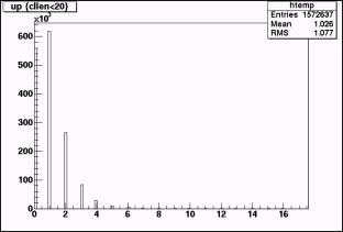
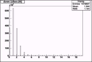
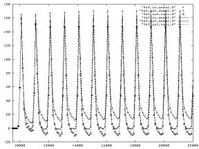
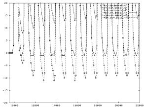
And here are the relationships between sequence max value and up&downstream hits.

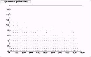
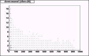
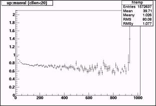
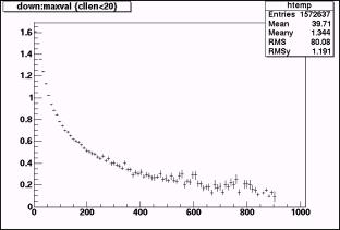
Almost all of the weight is in the 0, 1 & 2 bins for both upstream and downstream hits. Outside of these regions there is a very large spread (again, probably due to noise). Even so, the mean values of the up & downstream hits show reasonable distributions.

The upstream hit means are pretty much independent of the size of the hit, with a mean of ~.8. This is reasonable as the onset of the hit is very quick (the shaper time constant is ~1.9tb)

The downstream hits actually fall with the maximum hit. Larger hits have bigger undershoots, as well as bigger max values, but have roughly the same shape. The slope of the falling edge is greater, so statistically, fewer sequences will have a adc value fall in the 2 bucket range between 3-4.

These results suggest that the pre and post settings for the ALTRO zero suppression need not be large, and in fact that settings above 1-2 time-bins will do nothing but pick up additional noise.

Of course, there is an ultra-conservative ALTRO setting which should pick up all of the sequences found by the STAR asic: thresh = 1, seq = 2, pre = post = 0.

Similiarly, the ALTRO settings: thresh=4, seq=0, pre=1, post=2, should find every sequence that the current ASIC finds, although it could loose charge from the beginning and end of sequences compared to the ASIC.

The following table shows the occupancy, number of sequences and average sequence length for the current ASIC settings, as well as a number of ALTRO settings. For both the Altro and the STAR ASIC there is a distinction between the number of sequences determined by the hardware, and the number of sequences as defined by contiguous regions with adc > 0. In the case of the Altro, the number of contiguous regions is larger than the number of hardware sequences because the Altro combines sequences that are close together. In the STAR data, the effect is opposite, because a valley in a contiguous region which dips below thr_lo results in 2 hardware sequences. In the following table the contiguous regions are called “postproc” sequences while the hardware sequences are called “direct”.

Setting	Occupancy	Sequences (postproc)	Sequences (direct)	Len/sequence
ASIC seq_hi=0, seq_lo=2, thr_hi=4, thr_lo=1	3.95%	10709	10921	7.84
ASIC seq_hi=0, seq_lo=2, thr_hi=1, thr_lo=1	13.64%	62989	64650	4.57
ALTRO thr=4, seq=0, pre=0, post=0	2.74%	16622	16320	3.64
ALTRO thr=4, seq=0, pre=1, post=2	5.04%	17641	15049	7.26
ALTRO thr=1, seq=2, pre=0, post=0	14.24%	62740	54366	5.68
ALTRO thr=1, seq=2, pre=1, post=2	22.04%	80557	45613	10.47
ALTRO thr=2, seq=2, pre=0, post=0	4.04%	14849	14638	5.98
ALTRO thr=2, seq=2, pre=1, post=2	6.09%	16778	13883	9.51
ALTRO thr=2, seq=2, pre=0, post=1	4.74%	14767	14387	7.14
ALTRO thr=3, seq=2, pre=0, post=1	2.91%	7835	7756	8.13
ALTRO thr=3, seq=1, pre=0, post=1	3.46%	11377	11154	6.72

The immediate result is that the ultra-conservative approach (1/2/0/0) would lead to more than a 4-fold increase in the occupancy.

All of the clustering settings work fine for sequences large charge (Q>50 ADC). The only differences are in the way noise and very charge sequences are handled. These plots show the charge distribution of “postproc” sequences for various. The % in the legend is the occupancy.

The most promising setting is likely the 3/1/0/1 setting, which closely approximates the current ASIC for small Q sequences, but with a lower occupancy. If this is too stringent a cut on the low Q region, then 2/2/0/0 or 2/2/0/1 also give reasonable matches with minimal occupancy increases.

The following plot shows the Q distribution after zero suppression for simulated sequences. For this study phase of the hit with respect to the readout clock as well as the drift length was randomized.

The red line shows the integrated charge in the sequence after tail subtraction alone. This further demonstrates that the 3/1/0/1 ALTRO setting performance closely matches that of the current ASIC settings.

VI. Linearity of the Q Response

I wanted to check the linearity of the Q response for both the current ASIC and also for the ALTRO tail cancellation and zero suppression. To do this, I used simulated clusters. These results are also useful for the current STAR data to the extent that the ALTRO /PASA tail cancellation/shaping is similar enough to the current STAR. The simulated clusters had varying drift distance, phases with respect to the clock, and charges.

The first plot is the simple digitization effect of the ADC conversion. The green points are digitization by the value of the TPC pad response at the clock edge rather than the integration. The effect of the integration is to reduce the effect of digitization.

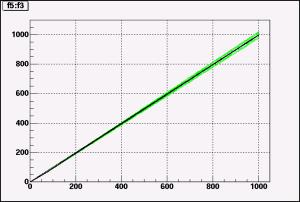
Digitization causes both non-linearity and noise in the measured charge. The non linearity is seen as a dip of ~8adc values, most pronounced for sequences at ~80 adc values. Also digitization causes an random noise of about +/- 3adc due to shifts in phase between pulse and digitization time.

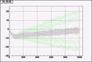
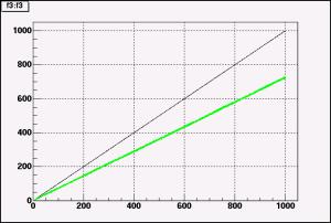
The ALTRO tail suppression algorithm has a significant effect on the charge. The resulting charge is shown in green and is about 72% of the charge without tail cancellation. The plot shows tail cancellation with optimal K values. The results for the calculated K values are very similar. Qaneal – Qcalc as a function of Q is shown on the right.

The tail suppression does introduce a small amount of non-linearity in the Q response. The following plots show the difference between charge after suppression and a linear response. (The left side is K by annealing, right side by calculation) A slightly stronger effect is shown with the hard tail suppression parameters.

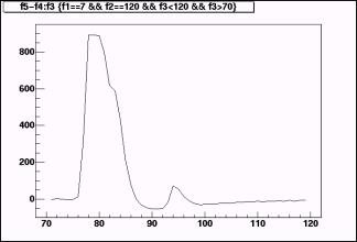
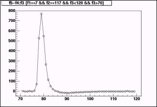
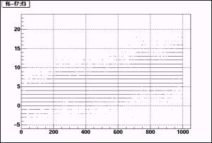
The following plots show the difference between charge after tail suppression and zero suppression from a linear response. On the left the 4/2/1/0 ASIC zero suppression is shown, on the right the 3/1/0/1 ALTRO settings are used. The effect of zero suppression is felt for Q < 20 where the efficiency for finding a sequence is significant. Surprisingly, however, once this region is passed, the zero suppression seems to correct the non-linearity seen after tail suppression alone. This might indicate that the non-linearities in the tail suppression come about from small shifts in the tails which are thrown away during zero suppression. The 3/1/0/1 ALTRO setting is nearly as good as the 4/2/1/0 ASIC setting at low Q and has lower occupancy.

For calculated tail suppression, the linearity is not restored as well.

References

Altro papers available at: http://ep-ed-alice-tpc.web.cern.ch/ep-ed-alice-tpc/papers.htm

1. ALICE TPC Readout Chip User Manual, http://ep-ed-alice-tpc.web.cern.ch/ep-ed-alice-tpc/altro_chip.htm

2. L. Musa et al., “The ALICE TPC Front End Electronics”, Proc. of the IEEE Nuclear Science Symposium, 20 - 25 Oct 2003, Portland

3. R. Campagnolo et al, “Performance of the ALICE TPC Front End Card”, Proceedings of the 9th workshop on Electronics for LHC Experiments, Amsterdam, 29 Sep - 3 Oct 2003

4. E. Beuville et al., “A Low Noise Amplifier-Shaper with Tail Correction for the STAR Detector”, Star Note 0230.

5. Altro Simulation, http://pcikf43.ikf.physik.uni-frankfurt.de/~tpc/Documentation/AltroSimulation.html

6. B. Mota et al, “Digital Implementation of a Tail Cancellation Filter for the Time Projection Chamber of the ALICE Experiment” in Proc, of the 6th Workshop on Electronics for LHC Experiments, Cracow, September 11-15, 2000