Hit-position errors in adjacent, outer-subsector pad rows are usually correlated in both X and Z; the sign and magnitude depend on pad-row crossing angle, dip angle and drift distance. We will discuss the correlations within the usual approximation, in which position resolution is subdivided into the three components:

• Base resolution: mostly uncorrelated, as long as the hit-position algorithms are not biased by where a track crosses a pad row, and the electronics noise is not correlated across rows. (Of course, the first is not true now, but this could be fixed.)

• Pad-row crossing angle: large anti-correlation in X.

• Dip angle: large anti-correlation in Z.

• Diffusion: moderate correlation in X and Z, due to anode wires coupling to more than one pad row.

We wish to demonstrate that such correlations complicate track fits and error assessments, even under ideal circumstances. We will not attempt to find detailed algorithms or parameterizations to deal with the complications, but will simply explore the effects in four cases:

• a) No correlations: ideal case (as usually assumed in STAR software).

• b) Large pad-row crossing angle: 45-degree, pad-row crossing angle; zero dip angle; Z=100 cm. Assumes 210-um base resolution, 175-um transverse diffusion, 13.5% coupling to each adjacent pad row, 1570-um contribution to hit residuals in X and an effective 100-um contribution by the hit to track errors.

• c) Large diffusion: zero pad-row crossing angle; zero dip angle; Z=0 cm. Assumes 210-um base resolution, 245-um transverse diffusion and 13.5% coupling to each adjacent pad row.

• d) Small pad-row crossing angle and moderate diffusion: 7.5-degree, pad-row crossing angle, zero dip angle; Z=100 cm. Assumes 210-um base resolution, 175-um transverse diffusion, 13.5% coupling to each adjacent pad row, 225-um contribution to hit residuals in X and an effective 100-um contribution by the hit to track errors.

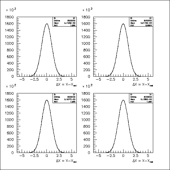
Hits were generated on 32 pad rows, using stand-alone (i.e., unofficial) software and the NORRAN random-number generator with correlations introduced for the four cases. To simplify comparisons, the distributions of hit errors were normalized to a mean of zero and a sigma of one. These normalized distributions of hit errors are identical, within statistics, as shown in Fig. 1. They correspond to hit errors with respect to the actual track (as opposed to a fitted track). For 32 hits, the distinction is modest, but will be explored later in this write-up.

Fig. 1: Hit errors were normalized to give gaussian-distributed, transverse hit errors with mean=0.000 and sigma=1.000; the four, 1-D error distributions are indistinguishable, within statistics.

If the 32 hits were independent, adding their errors and dividing by 32 would yield another Gaussian distribution, reduced in width by a factor of 1/sqrt(32)=0.1768. The actual results are shown on the same scale in Fig. 2, where only the uncorrelated distribution in Fig. 2a behaves "properly." Anti-correlations tend to cancel the hit errors beyond the level expected for randomness, accounting for the narrowness of Fig. 2b, while positive correlations do the opposite in Fig. 2c. In Fig. 2d, the positive correlation has nearly cancelled the anti-correlation, leaving a distribution that is only slightly narrower than that for random hits.

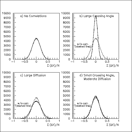
Fig. 2: When 32 gaussian-distributed, transverse hit errors are averaged, correlation effects are made visible -- a large anti-correlation in (b), a modest positive correlation in (c), and a small anti-correlation in (d). The uncorrelated distribution from (a) is superimposed on the other plots for comparison.

Hit correlations will also affect the chi-squared/degree-of-freedom distributions, since the probability of an error is related to that on adjacent pad rows. The effect of assuming 32 degrees of freedom is shown in Fig. 3: the high and low tails are elevated for both Fig. 3b and 3c. The distribution in Fig. 3d for the almost uncorrelated case almost matches the "correct" distribution in Fig. 3a.

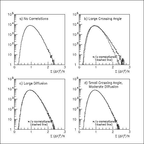
Fig. 3: "Chi-squared/degree of freedom distributions" for N=32 hit errors relative to the real track. In all cases, the mean of the distribution is 1.0, but correlations (positive or negative) increase its width. This is especially visible with the strong (anti-)correlations in (b). The true chi-squared distribution from (a) is superimposed on the other plots for comparison.

If the naive chi-squared/d.o.f. distributions of Fig. 3 are converted to confidence level, the distributions will not be flat when there are net correlations. The effect is seen in Fig. 4. The distributions are affected, but not flattened, if one replaces 32 by some other number of d.o.f.

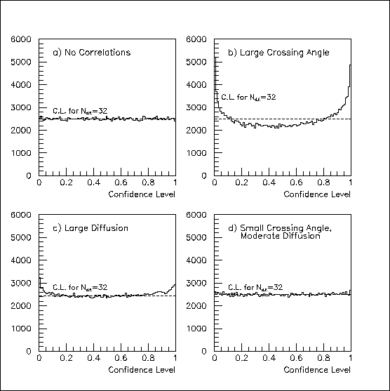
Fig. 4: The "chi-squared/degree of freedom distributions" for N=32 hit errors from Fig. 3 translate into the confidence-level distributions shown. The non-statistical deviations from flatness in (b), (c) and (d) result from the pad-row correlations.

The degree-of-freedom problem becomes even murkier when we fit a track to correlated hits. For purposes of illustration, 2-D tracks were fit to the 32 simulated, outer-sector hits. In the absence of correlations, the chi-squared/32 distribution is shifted to lower values, as shown in Fig. 5a. The shift is smaller if the hits are anti-correlated, and is tiny for Case b, as shown by Fig. 5b; this is because the residuals are so much larger than the effective hit errors. Conversely, the shift is larger for positively correlated hits, as in Fig. 5c.

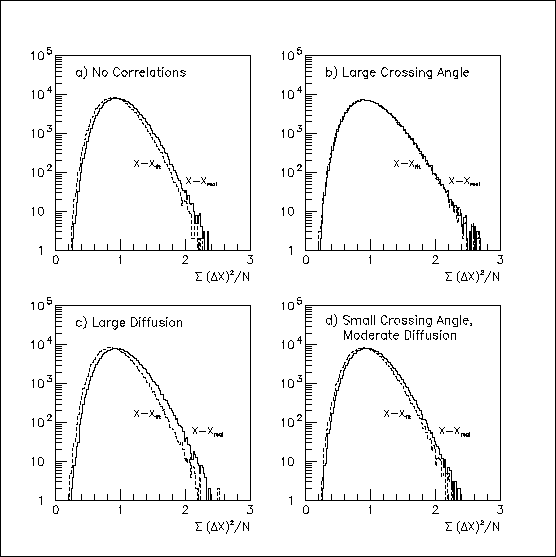
Fig. 5: The solid lines reproduce the plots from Fig. 3 that show the "chi-squared/degree of freedom distributions" for N=32 hit errors relative to the real track. The distributions shown by dashed lines also (incorrectly) assume 32 degrees of freedom, but are for the errors relative to a 2-D track fitted to the hits projected onto the X-Y plane.

In the case of uncorrelated hits, one can convert chi-squared to confidence level for N=32-2=30 degrees of freedom; the result is, of course, flat, as in Fig. 6a. With correlated hits, there isn't an especially good choise, though somewhat symmetrical distributions are obtained in Fig. 2b for N=31, and in Fig. 2c for N=29. Of course, N=30 works fairly well for Fig. 2d.

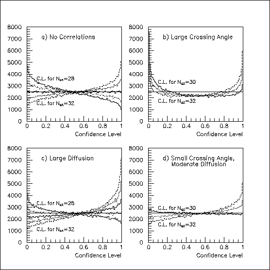
Fig. 6: The "chi-squared/degree of freedom distributions" relative to a fitted 2-D line from Fig. 5 translate into the confidence-level distributions shown for various assumption about the number of degrees of freedom. Without correlations, as in (a), there are N=32-2=30 degrees of freedom, as expected, and this is also a good approximation in (d). With the large anti-correlations in (b), there really isn't a good value, but N=31 is the best of the bad choices. For the modest correlations in (c), N=29 works fairly well.

Strictly speaking, chi-squared is defined only in the absence of correlations. One can imagine removing known correlations, but the event-to-event variation in the TPC pad-row correlations is large and there is significant lost information; correcting for the average correlation with adjacent pad rows only makes matters worse (unfortunately). I don't know of a clean way to correct for the correlations analytically; in the end, one may be forced to parameterize corrections using Monte Carlo results. However, neither Trs nor tfs are up to this task, as of early April, 2000.

There are several obvious places in the STAR analysis chain where problems might arise from ignoring the correlations between pad rows:

1. tfs: If the fast simulator produces hits which reproduce the correct distribution of residuals, while ignoring the correlations, the tracks later fitted to these hits will not correctly reproduce the real resolution. This is not necessarily a small effect. (In principle, if not yet in practice, trs would automatically incorporate most correlations; within the current design of tfs, they would have to be incorporated by hand.)

2. Hit Rejection: The meaning of "outlier" is modified in the presence of strong correlations: if the pulls from adjacent hits largely cancel, it may be worse to reject an apparent outlier than to retain it. Excepting extreme cases, outliers can't be analyzed in isolation.

3. Track Fitting: Even tracks fitted to hits sampled from the correct distribution (real data or accurate Monte Carlo) will have less than optimal resolution if the hits are not assigned correct weights in the fit. This is even true for straight tracks where weights for all hits in the inner subsector, and for all hits in the outer subsector should be nearly the same --- since the weights in the inner and outer subsectors are unlikely to be off by the same factor.

4. Track Error Estimation: If the effective errors of the hits are wrong at the factor-of-two level, one will have a biased estimate for the uncertainties of the fitted momentum and projected track.

5. Track Rejection: If tracks are rejected due to a low "confidence level," one will probably have to deal with a non-flat confidence-level distribution --- cutting below the 10% C.L., for example, may not reject 10% of the tracks.

6. Global: There is a conflict between the desire to pass highly distilled data to the global fitting routines, and the need to deal with complicated, TPC-specific issues; one cannot distill TPC hit down to a hit position and an error.

For the simulated, straight tracks discussed above, the first effect was usually the dominant one. The distributions of track parameters fitted with naive error estimates were only a few percent wider than the optimal ones. However, fits of curved tracks are more sensitive to the end points (with resolution scaling as 1/[L^2 * sqrt(N+4)]), so this should be revisited with Trs when possible.

Written: R.Bossingham (5-April-2000).

The issue of anti-correlated hits in adjacent pad rows of the STAR TPC was originally pointed out, I believe, by Howard Wieman. Also, I would like to acknowledge useful discussions with several other people in STAR --- Al Saulys, Iwona Sakrejda and Spencer Klein come immediately to mind. I regret the inevitable omissions.