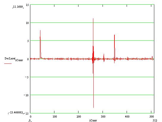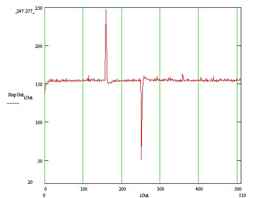
Raw data measured pulsing the ground plane with a step function. The rise and fall of the function clearly show up.
This is an ongoing works. There are probably
many mistakes on this page, and things that are unclear, so please
comment.
For more details about the purpose of these measurments see the STAR TPC pages
Pulsing the ground plane
To calibrate the signal amplitude, we pulse the ground plane. We expect to induce on the pads, a signal that is the derivative of the pulser output. However, we cannot make sure that the waveform is properly differentiated. There are many potential sources of problems: cable lengths, anode wires...
We can see the signal that we readout pulsing
the ground plane as a convolution of 3 functions:
PulserSignal(t) = Waveform(t) * Unknown(t)
* FEEResponse(t)
The Unknown(t) component is thought
to be a perfect differentiator
Since it cannot be checked, we rewrite
the transformation as
PulserSignal(t) = d/dt(Waveform(t))
* Unknown2(t) * FEEResponse(t)
Unknown2(t) may be equal to the
identity.
With this expression, when we pulse the
ground plane with a step function we measure the response function:
Unknown2(t) * FEEResponse(t)
Here are some data taken pulsing the ground plane with a step function :
Raw data measured pulsing the ground plane with a step function. The rise and fall of the function clearly show up.
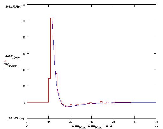
Response to the rise of the step function.
The fit is performed using the following
function:
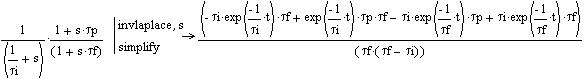
This function doesn't reproduce the rise of the signal. However it accounts for the tail cancellation and the preamplifier response.
Using a step function, it is clear that we will never get a perfect delta function even if the unknown part is equal to 1. We assume that the width of the signal we get using the step function is small compare to the time scale of the measurment. Thus it can be treated as a delta function. Lanny Ray sugested to measure the delta reponse pulsing the ground plane with waveforms having finite (and known) widths, and to extrapolate to zero. At some point it should be done as a consistency check.
Shape of the laser signal
The laser signal shape can be easly study
since the cluster are always at the same place. We can average over several
events to get the time shape of a laser signal. The only difference between
the laser and the true particle is the ionisation. Thus it compares well
to low deep angle tracks.
100 laser events were taken reading out
a single board.
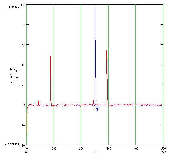 Laser signal on 1 pad. The response function to a step function on the pad plane is shown for comaprison
Now we can deconvolute the laser signal by the response function. This way we get the time shape of the laser pulse before being shaped. The result of the deconvolution is shown below.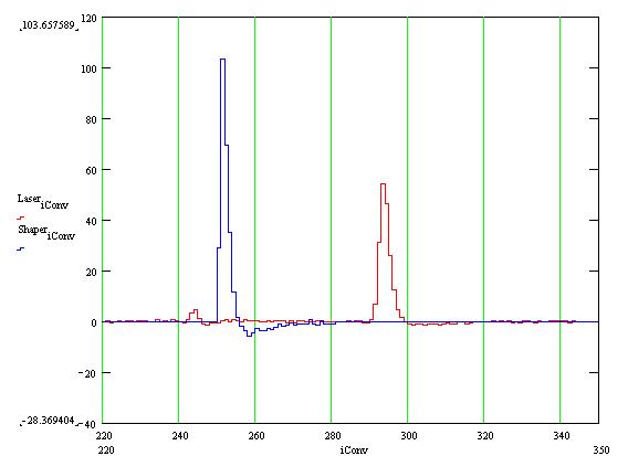 Zoom to the same plot : blue : Electronic response function, red : laser pulse
The large peak around 260 must be ignored. The time bucket zero of the original laser signal is shifted to 260 due to the fft deconvolution method. We see clearly the 2 main laser peaks.
Here, we compare the convolution result with calculation from a macroscopic model. The deconvoluted signal is much narrower than the model predict. There are two (more?) explanations :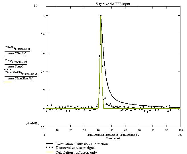 Zoom to the first peak : dot. For comparison calculation results are shown.
The main idea of this pulser calibration is to put at the input of the FEE, a signal that will fake the one from real tracks. For the time being, we try to fake a laser signal. To do so, we don't need to understand the shape of the deconvoluted function. We will pulse the ground plane with the integrated deconvoluted laser function. Below, pulser waveforms that we use, are displayed.
The results are shown below.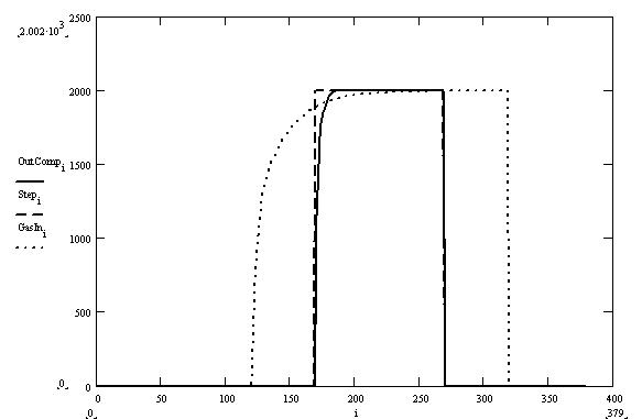
Wavetek output waveforms : The solid line is the integrated deconvoluted laser function. the dot line is the integrated function calculated using the macroscopic model. The dash line is the step function.
Both curves compare rather well. However, the shape of the laser is not constant from one shot to the other. Depending on the cluster, one chose the agreement between the laser shape and the pulser one may get worse. For the time being, we will use the waveform calculated above.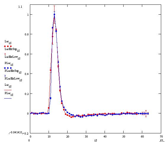
FEE response to a laser shot in red and pulsing the ground plane with the integrated deconvoluted laser function, in blue.
Calibration curve
Varying the amplitude of the pulse one
can draw a calibration curve. The question is : should we use the area
of the signal or its peaks? we compared both method pulsing the ground
plane with a step function. In a next future we will redo the same analysis
with the "laser like" pulser waveform.
It seems that the peak measurement is the most stable, i.e. linear. The area of the non zero supressed data is sensitive to the undershoot. However, on the gas data, the undershoot is very small.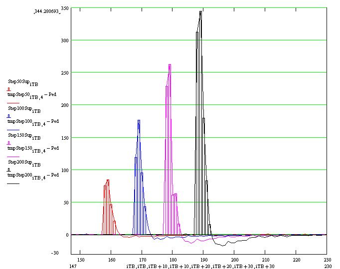
FEE response to a step function. The bars show the amplitude of the time buckets that remain after zero supression. Amplitude : red 50 mV, blue 100 mV, magenta 150 mV, black 200 mV
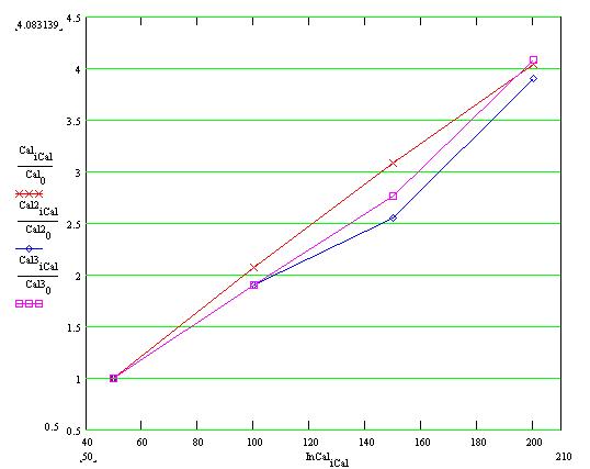
Cluster amplitude (arbitrary set equal to 1 at 50 mV input) versus the pulser amplitude (in mV).
Red : peak calculation, blue : area calculation, magenta : area calculation for zero supressed data.