Reconstruction of Track Candidates

In this step CATS creates track candidates out of space-points and collects hits missed in layers where space-points could not be reconstructed due to dead regions or detector inefficiencies.

The first task is fulfilled by a cellular automaton, which uses space-points as input elementary units or cells. A cellular automaton is a discrete-time dynamical system that evolves in a phase space consisting of cells. Lets denote the space-points as $s_{ij}$, where $i$ is the number of superlayer, $i=1,\dots,N$, $j$ is the number of a space-point inside $i$-th superlayer and each space-point is defined by a set of its parameters: $s=\{x,y,t_x,t_y\}$. At any moment $k$ of discrete time, each cell (or space-point) can take several states $p^{k}_{ij}=\{1,2,\dots, N\}$. The automaton's evolution, i.e. evolution of the cell states, is determined by a set of rules (for instance, a table) according to which the new state of a cell is calculated on the basis of the states of its neighbors in the next and previous superlayers. The final value of a state $p^{n}_{ij}$ is equal to a position of the space-point $s_{ij}$ on a reconstructed track candidate. All initial states $p^0_{ij}$ are assumed to be equal unity.

After initialization the cellular automaton performs the following loop over superlayers $L=2,\dots,N$, starting with the second superlayer, $L=2$:

1. For each space-point $s_{Lj}$ the automaton finds its neighbors in the previous superlayer $L-1$. A space-point $s_{L-1,l}$ is regarded as neighboring if
   $$D(s_{ij},s_{L-1,l})\le D_{max},$$
   where ${D}(\cdot,\cdot)$ is a $\chi^2$-distance between two space-points, ${ D}_{max}$ is a predefined cut.
2. If a neighbor is found, the new value of the state $p^{k}_{Lj}$ is calculated as follows
   $$\widetilde{p}^k_{Lj}=p^k_{Lj}+ \left\{ \begin{array}{l} 1, \... ...t] 0, \mbox{ if } p^k_{L-1,l}\ne p^k_{Lj} \end{array}\right. .$$

3. When the automaton calculates new states for all space-points in all superlayers, the states are updated simultaneously and the algorithm proceeds with the next iteration:
   $$p^{k+1}_{Lj}=\widetilde{p}^k_{Lj}, \qquad k=k+1, \qquad L=2,\dots,N.$$

If, during an iteration, all states keep their values, the automaton stops the iteration and proceeds with the collection of track candidates:

1. The algorithm starts with space-points for which $p^n_{ij}=N$.
2. If they exist, the algorithm finds a neighbor for each such space-point in the previous superlayer so that
   $$p^n_{i-1,l}=p^n_{i,j}-1.$$

3. If such a neighbor exists, the algorithm tries to find its neighbor in the $(i-2)$-th superlayer and so on, creating a branch or track candidate.
4. If, in some superlayer, more than one neighbor is found, the algorithm splits the candidate into two branches which are then propagated independently.
5. The collection of a track candidate is completed if the algorithm found a neighboring space-point with $p^n=1$.

When all branches starting with states $p^n_{ij}=N$ are completed, the algorithm proceeds with the remaining space-points with lower states $p^n_{ij}=N-1$, and so on.

All collected track candidates are refitted by the Kalman parameter estimator, candidates with a bad $\chi^2$ are discarded.

Further details on the application of cellular automata for track searching can be found in [#!CATS-NIM!#].

Figure 4.5: Track candidates reconstructed by the cellular automaton after the track following procedure.

The clear advantage of a cellular automaton is its intrinsic simplicity which makes tracking based on it extremely fast. Unfortunately, the search for tracks performed by a cellular automaton is not exhaustive, for example, if, in an intermediate superlayer, there is no neighboring space-point, the cellular automaton cannot jump over such a hole. This problem is typical in case of dead regions in the OTR.

Due to this reason, in CATS, the tracking based on a cellular automaton is accompanied by a simple (and fast) track following procedure. As seeds, this procedure uses track candidates found by the cellular automaton and space-points for which the automaton could not find any neighbors.

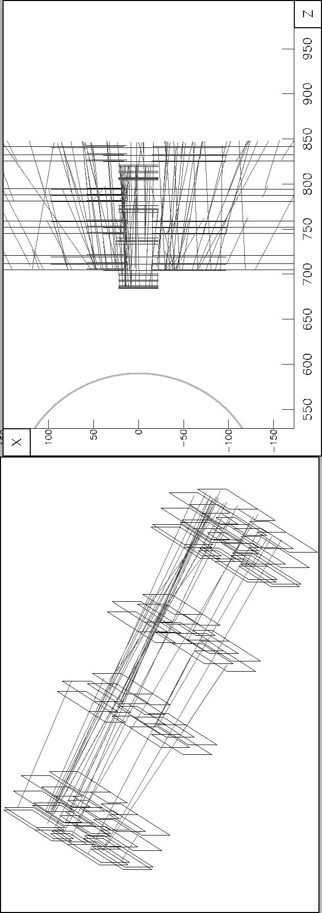
A special track following procedure is also used for propagation of track candidates reconstructed in the ITR into the Outer Tracker. Since the hit resolution of the ITR is much better than for the OTR, it is possible to resolve L/R ambiguity ``on the fly'', i.e., in the course of the track following. Therefore this particular procedure works with the OTR hits rather than clusters of hits. An example of the picture obtained at this step of the CATS reconstruction chain is shown in Fig. 4.5.