The wiremap is a distribution which contains the positions of all
strips belonging to clusters. The mean wiremap is the wiremap
normalized to the number of processed events and to the rate. The
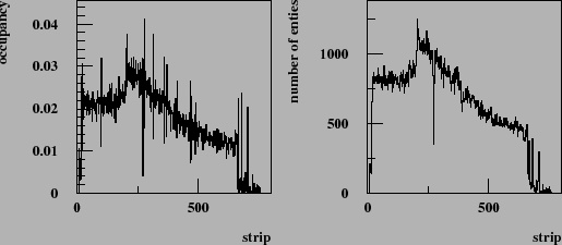
occupancy consists of the clusters' center of gravity
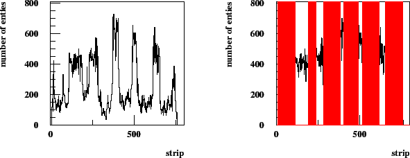
positions normalized to the number of events. The example of an occupancy
and a wiremap is shown in Fig. 5.1. The overall shape
is determined by the beam pipe cut-out and the radial decrease of particle
density.
At first glance occupancy and wiremap look almost the same, but the wiremap
has several advantages: it allows to locate problematic channels more easily,
which could not be used during clusterization, and it increases the accumulated
statistics by a factor of about 3.
Figure 5.1:
On the left, occupancy for chamber MS01++4.
On the right, wiremap for chamber MS01++4.
 |
The masking procedure is based on the assumption that the average hit density of a single
chamber does not deviate too much from the average hit density of the station.
The average hit density of the station is defined as the sum of the wiremaps
of all chambers in one superlayer normalized to the number of events,
the rate and the number of chambers in the station.
We can subdivide the procedure into the following steps:
- In order to find completely dead chambers, the average hit density of an
investigated chamber
 is compared to the average hit density of the station
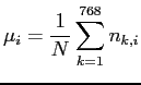
 . The average hit density for the chamber
  can be written as
 |
(5.1) |
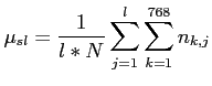
and for the station
 |
(5.2) |
 is the number of times charge is deposited on
a strip
is the number of times charge is deposited on
a strip  of a chamber . The value
  denotes the number of chambers
in the particular station and
denotes the number of chambers
in the particular station and  is the number of processed events. If the
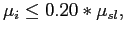
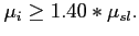
average hit density of a chamber is below 20%
of the average hit density,
is the number of processed events. If the
average hit density of a chamber is below 20%
of the average hit density,
 |
(5.3) |
of the station all channels are marked as dead.
In case it is above 140% all channels are marked as hot
 |
(5.4) |
All chambers which are not hot and dead are further considered at steps 2 and 3.
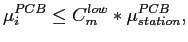
- At the next step, the search for dead and hot PCBs5.1 among the remaining chambers is done.
A sketch showing the distribution of PCBs over the chamber is shown in Fig.
5.3. The hit densities for each single PCB are accumulated and
three average hit densities of a station (for each PCB) are calculated.
The hit density thresholds are optimized in order to take into account
the shape of the wiremap:
- low
 =30%, high
 =150 % for PCB A
- low
 =50%, high
 =180 % for PCB B
- low
 =20%, high
 =140 % for PCB C
According to the following condition PCBs are marked as dead, hot and normal.
 |
(5.5) |
 |
(5.6) |
The value  denotes the type of PCB: A, B or C.
- Finally, single strips are considered.
For each strip, the average number of hits is calculated.
The average hit densities of the
PCBs in similar positions in one station5.2 are calculated and normalized to the number of strips
(256 stips are connected to one PCB). If the hit density of the strip is below
20% or higher than 140% of the average hit density of this PCB then the strip is marked as dead respectively as hot.
Figure 5.2:
On the left, wiremap for chamber MS01++4.
On the right, wiremap with dark color masked strips are shown for chamber MS01++4.
 |
In order to produce masks for all chambers in one run, a sample of
approximately 10.000 events is needed.
Only runs without problems were considered.
For some runs the stability of the Inner Tracker high voltage
during data taking was checked. Masks have been produced for most of
the minimum bias and triggered runs in 2002 - 2003.
Figure 5.3:
Sketch of an ITR chamber indicating the distribution of
PCBs over the chamber.
 |
The mean number of masked strips in runs of 2002 are shown in
table 5.1.
The time period between the run 200965.3 and 21072 is approximately four months.
Fig. 5.2 shows on the right the mask produced with the described
masking procedure overlaid on top of the associated wiremap.
Table 5.1:
Percentage of masked channels in the inner
tracker system. The first and the last eight not connected strips are not counted
(dead chambers are included).
| Station |
run 20096 |
run 21072 |
| MS01, % |
7.1 |
8.8 |
| MS10, % |
50,35 |
53.68 |
| MS11, % |
16.54 |
16.87 |
| MS12, % |
14.2 |
16.62 |
| MS13, % |
60.28 |
61.30 |
| MS14, % |
-- |
18.8 |
| MS15, % |
-- |
57.6 |
The obtained masks are stored in the Data Base.
During running in 2002-2003 several chambers in the Inner
Tracker system have shown a rather bad performance. A typical
wiremap for one of the problematic chambers is shown
in Fig. 5.4.
Figure 5.4:
On the left, a wiremap for chamber MS10++4.
On the right, a wiremap with masked strips shown in dark color for chamber MS10++4.
 |
It was found that the resistance between neighboring strips on the Kapton Fanin
which connects MSGC and Frontend electronics was too low. It seems that the
reason for this behavior is due to the glue or the glueing procedure,
used for bonding the chamber to the PCB [#!itrloss!#].
Fig. 5.4 shows a wiremap and the mask for an
affected chamber.
The distribution on Fig. 5.4
at the right shows the masked channels (dark) overlaid on top of the
wiremap of the chamber. These masked regions have to be excluded for
the determination of the pure efficiency.
Yury Gorbunov
2010-10-21