As already noted, using Kalman filtering techniques is one of the basic
principles of the CATS track reconstruction strategy. The Kalman filters and Kalman-type
parameter estimators are embedded in
- space-point parameter estimation during space-point reconstruction;
- propagation of track candidates through empty superlayers and gathering of
missed hits during the track following procedure;
- outlier detection and elimination;
- smoothed refit of reconstructed segments. This
refit includes the treatment of multiple scattering effects using a preliminary
estimate of the track momentum. It is the final step of track reconstruction.
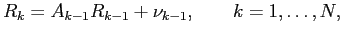
The Kalman filter addresses the general problem of trying to estimate the
state vector  of a discrete-time process that is governed by the
linear stochastic difference equation
of a discrete-time process that is governed by the
linear stochastic difference equation
 |
(4.1) |
where the matrix  relates the state at step
  to the state at step
  .
.
 is a process noise, a sequence of independent Gaussian variables
which can, for example, account for the multiple scattering influence on the state
vector. Within the model (4.1) a track in the Pattern Tracker can be
described as a straight-line motion in the presence of Gaussian disturbances:
is a process noise, a sequence of independent Gaussian variables
which can, for example, account for the multiple scattering influence on the state
vector. Within the model (4.1) a track in the Pattern Tracker can be
described as a straight-line motion in the presence of Gaussian disturbances:
 |
(4.2) |
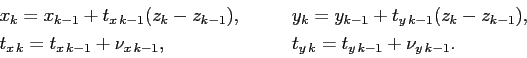
The state vector
 describes the
track parameters taken at the detector plane with
describes the
track parameters taken at the detector plane with  .
.  denotes transposition,
the random variables
denotes transposition,
the random variables
 ,
,
 describe the influence of multiple
scattering on the track when it passes through detector plane ,
describe the influence of multiple
scattering on the track when it passes through detector plane ,
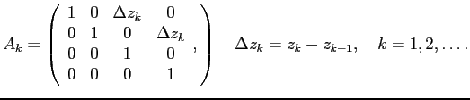
 . According to the track model (4.2), the matrix
  in
equation (4.1) has the form
in
equation (4.1) has the form
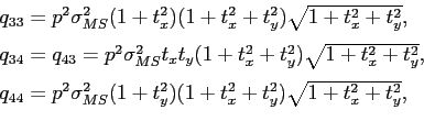
In CATS the detector volumes and insensitive walls are treated as so-called
thin scatterers [#!ranger!#]. For such scatterers, the non-zero elements
 of the covariance matrix
  of the noise vector
 equal to
where  is an external estimate of the inverse momentum of the particle,
 is the mean variance of the multiple scattering angle for
a 1 GeV particle.
is the mean variance of the multiple scattering angle for
a 1 GeV particle.
The input to the filter is a sequence of measurements  which are described by a linear function of the state vector
 |
(4.3) |
where the matrix  in the measurement equation (4.3) relates
the state to the measurement
in the measurement equation (4.3) relates
the state to the measurement  ,
,  is a sequence of Gaussian random
variables with the covariance matrix
is a sequence of Gaussian random
variables with the covariance matrix  .
.
The ITR and OTR have different measurement models. In addition, the OTR
measurement model needs linearization. The matrix for the ITR reads:
where  is the rotation angle of the strips in the ITR plane .
The linearized measurement matrix for the OTR has the form:
is the rotation angle of the strips in the ITR plane .
The linearized measurement matrix for the OTR has the form:
where is the rotation angle of the sensitive wires in the OTR plane ,
and
where  is the
  -coordinate of the -th wire in the rotated coordinate
system.
-coordinate of the -th wire in the rotated coordinate
system.
Let's define
 to be a state estimate at step after
processing measurement . The main idea of the Kalman filter is that
the optimal (in mean-square sense) estimate
should be the sum of an
extrapolated estimate
to be a state estimate at step after
processing measurement . The main idea of the Kalman filter is that
the optimal (in mean-square sense) estimate
should be the sum of an
extrapolated estimate
 and a weighted difference between an actual
measurement and a measurement prediction
and a weighted difference between an actual
measurement and a measurement prediction

where
The matrix  is called the filter gain and is chosen to minimize the
sum of diagonal elements of an estimation error covariance matrix
is called the filter gain and is chosen to minimize the
sum of diagonal elements of an estimation error covariance matrix
 .
By definition,
.
By definition,
where E denotes the mathematical expectation.
Note, that for both detectors, OTR and ITR, the measurement models are scalar.
In this case the minimization leads to the following formula
for
where
 is
the extrapolated estimation error covariance matrix
is
the extrapolated estimation error covariance matrix
 . The formula for
follows from equation (4.1):
. The formula for
follows from equation (4.1):
The new minimized value of the error covariance matrix
is defined
by the equation
where  is the unity matrix.
The computational algorithm of the discrete Kalman filter consists of two steps:
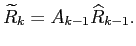
- Prediction step -- extrapolation of the estimate
 and the error
covariance matrix
and the error
covariance matrix
 to the next step of the algorithm.
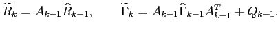 |
(4.4) |
- Filtering step
- the gain matrix calculation
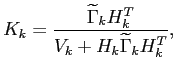 |
(4.5) |
- the updated estimate
|
(4.6) |
- the updated error covariance matrix
 |
(4.7) |
The two steps, prediction and filtering, are repeated until all
measurements are processed.
In order to speed up the CATS reconstruction procedure, all fitting routines are
written using the optimized numerical implementation of the Kalman filter algorithm
described in [#!CATS-NIM!#]. In general, there are several ways to reduce the
computational cost of the standard Kalman filter/smoother algorithm:
- calculate the covariance matrix in triangular form taking its
symmetry into account;
- optimize the procedure to update the covariance matrix.
The most time-consuming parts of the filtering step are the calculation of the gain matrix
and the updated covariance matrix. Let's rewrite (4.5) as follows
where the vector  and the scalar
  are
are
In terms of and the filtering step can be simplified.
The optimized update of the triangular covariance matrix reads
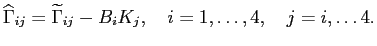 |
(4.8) |
In order to get smoothed estimates at each point of a track, CATS
employs the standard backward Kalman smoother. The smoother is an recursive algorithm
that starts with the last point  and updates the estimates and their covariance
matrix at the next point
and updates the estimates and their covariance
matrix at the next point  using the estimates and the covariance matrix
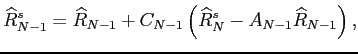
given by the Kalman filter at the last point. The update of the estimate
using the estimates and the covariance matrix
given by the Kalman filter at the last point. The update of the estimate
 is described as follows
where superscript ``s'' denotes a smoothed value,  is the smoother gain
given by the equation
is the smoother gain
given by the equation
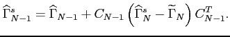
The calculation of requires the inversion of
the  symmetrical matrix
 at each point. The smoothed
covariance matrix reads
at each point. The smoothed
covariance matrix reads
By definition
 and
and
 .
After updating point the smoother proceeds with point
.
After updating point the smoother proceeds with point  and so on
until it reaches the first point
and so on
until it reaches the first point  . To update the -th point the smoother
uses smoothed values of
. To update the -th point the smoother
uses smoothed values of
 and
and
 already calculated
at the previous,
already calculated
at the previous,  -th, point.
Yury Gorbunov
2010-10-21
![$\displaystyle H_k=\Bigl[\cos\alpha_k, \:-\sin\alpha_k, \: 0, \: 0\Bigr],
$](img214.png)
![$\displaystyle H_k=\frac{1}{\sqrt{1+t_{uk}^2}}
\Bigl[\cos\alpha_k, \:-\sin\alpha...
...cos\alpha_k}{1+t_{uk}^2} ,
\:\frac{\Delta u_k\sin\alpha_k}{1+t_{uk}^2}\Bigr],
$](img216.png)
![$\displaystyle \widehat{\Gamma}_k={\bf E}\Bigl[(R_k-\widehat{R}_k)(R_k-\widehat{R}_k)^T\Bigr],
$](img226.png)