Next: MC and Data Comparison Up: Inclusive Production Cross Sections Previous: Acceptance Contents
In HERA-B several methods for luminosity determination
are available [#!Lumi!#]. The algorithms used for luminosity
determination of minimum-bias data taken in 2002/2003 are discussed
in this section.
The luminosity ![]() is the number of particles passing down the line per
unit time, per unit area, and can be expressed as:
is the number of particles passing down the line per
unit time, per unit area, and can be expressed as:
 |
(6.6) |
 |
(6.7) |
 |
(6.8) |
where
![]() indicates how many times filled bunches crossed the target region
and
indicates how many times filled bunches crossed the target region
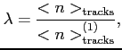
and ![]() is the mean number of interactions for filled bunches.
is the mean number of interactions for filled bunches.
For the luminosity determination of the minimum bias data of 2002/2003 three different methods were used:
Hodoscope counters
The rate in the HERA-B setup 2002/2003 was measured by four pairs of scintillators,
placed symmetrically around the beam pipe. Each counter has a geometrical acceptance equal to
approximately 0.15%. The acceptance of these counters has been calibrated relative
to a large acceptance hodoscope (![]() 54% acceptance). This large acceptance
hodoscope was temporary installed inside the magnet. Interaction rate measured by the
hodoscope counters can be expressed as follows
54% acceptance). This large acceptance
hodoscope was temporary installed inside the magnet. Interaction rate measured by the
hodoscope counters can be expressed as follows
 |
(6.9) |
ECAL Energy Sum
The idea behind this method is that average energy measured in the ECAL proportional to the mean number of superimposed interactions.
The average energy ![]() deposited by events with exactly
deposited by events with exactly ![]() interactions
is
interactions
is
 |
(6.10) |
 |
(6.11) |
 |
(6.12) |
The assumed linearity of the ECAL energy with respect to the number of interactions was checked by a Monte Carlo simulation and verified with experimental data. A typical distribution of the average energy dependence on the interaction rate for two wire materials carbon and titanium, obtained on data, is shown in Fig. 6.9.
The energy of a single interaction can be determined from MC or data. A single
interaction can be tagged in the zero-rate limit (at low rate the probability to have
multiple interactions becomes negligible small), by requiring at least one cell with energy
above threshold, such event is called ``tagged'' event. Taking into account the
assumption that the number of interactions follows the Poisson statistics, the mean
energy per tagged event can be defined as a function of the parameter ![]()
where
![]() is the efficiency to tag an event (measured on MC),
is the efficiency to tag an event (measured on MC), ![]() is
the energy released with one interaction [#!Asom!#]. The energy
is
the energy released with one interaction [#!Asom!#]. The energy ![]() is obtained
from a fit to the mean energy of tagged events using function 6.13
is obtained
from a fit to the mean energy of tagged events using function 6.13
Vertex Detector System based method
As an additional method the response of the Vertex Detector System is used. Assuming
that the number of reconstructed tracks and vertices scales linearly with the
number of interactions ![]() , we can express
, we can express ![]() in a similar way
as in the case of the ECAL energy sum method
in a similar way
as in the case of the ECAL energy sum method
 |
(6.14) |
The obtained numbers (
![]() ) are used to
calculate the total number of filled bunches which crossed the target region and to
correct the efficiencies of the applied cuts. The
) are used to
calculate the total number of filled bunches which crossed the target region and to
correct the efficiencies of the applied cuts. The
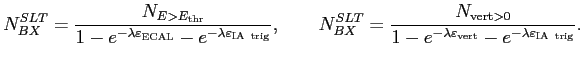
![]() for each of the
methods can be expressed as follows
for each of the
methods can be expressed as follows
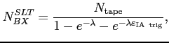 |
(6.15) |
where ![]() is the average number of interactions determined with the Hodoscope counters,
is the average number of interactions determined with the Hodoscope counters,
 |
(6.16) |
The numbers obtained with the different methods were compared for a set of runs for
different wires. The results of the comparison are shown in Fig. 6.10 for Tungsten
wire. The measurements obtained with the ``mean'' and ``Poisson'' method are in
good agreement. The estimated systematic error of the luminosity measurements
is ![]() 10%. The final luminosity numbers used in the analysis are listed in
Appendix A.
10%. The final luminosity numbers used in the analysis are listed in
Appendix A.
Yury Gorbunov 2010-10-21