Kopytine's homepage

Amplitude calibration of the Si channels

Amplitude calibration was carried out channel by channel for all 512 channels. The following elements are essential to understand the procedure.

1. Using a given run ( $4\times10^4$ events), we accumulate a histogram of amplitudes for a given channel. A typical distribution is shown on Fig.  6.1

   Figure 6.1: A typical calibration fit. Channel 1.

   

2. Normalize the amplitude distribution to unit total integral. The same normalization is imposed on the fitting model in the calculations. This removes one fit parameter, but requires extra work in figuring out and imposing the normalization of the fitting function.

3. Empty pad peak. The fitting function was developed by using data from a valid beam trigger run (low multiplicity).

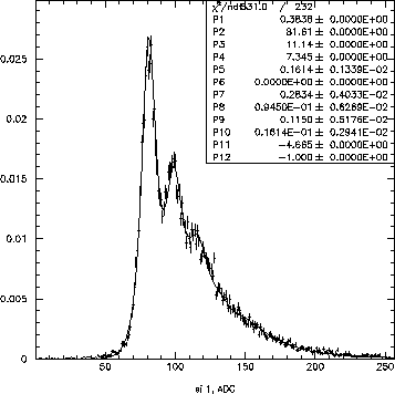
   Its distribution represents noise inherent in all signal measurements. Therefore, in the fitting model, this noise distribution is folded with physical fluctuation of the ionization energy loss. The shape of the peak is non-Gaussian; it has somewhat more events on the tails. Therefore, I describe this peak by a product of a Lorentzian (a function with pronounced tails), and a Gaussian which prevents those tails from going too far. The noticeable asymmetry of the peak is taken into account in two ways: by introducing an addition of an odd-power Hermite polynomial (with $p_{11}$) and by displacing the symmetry axis of the Lorentzian with respect to that of the Gaussian (through $p_{12}$).

   $$\mathcal{N}\mathnormal(x) = \frac{1}{n}\frac{\exp(-\frac{1}{2}(\f... ...frac{p_{11}}{p_3})^3(8(\frac{x}{p_3})^3-12\frac{x}{p_3}) }{(x-p_{12})^2+p_4^2}.$$ (56)

   
   

   The normalization constant $n$ has to be calculated numerically. $x_0= x-p_2$, where $x$ is the ADC channel number and $p_2$ is the position of the empty pad peak.

4. Ionisation energy loss is a random process and large fluctuations can occur in the energy $\,dE$ deposited by a particle in a layer of material. The thinner the layer, the more pronounced is the tail of the statistical distribution of $\,dE$. This is characterized by the parameter

   $$\kappa = \frac{\xi}{E_{max}},$$ (57)

   
   
   where $\xi$ is the mean energy loss of a particle with charge 1, moving with velocity $\beta$, and undergoing Rutherford scattering on an atom with atomic mass $A$, and $Z$ electrons, in a medium of such atoms of thickness $t (g/cm^2)$:

   $$\xi = \frac{153.4 Z t}{A\beta^2} keV.$$ (58)

   
   

   $E_{max}$ is the kinematical upper limit on the energy transfer in a single collision:

   $$E_{max} = \frac{2m_e\beta^2\gamma^2}{1+2\gamma m_e/M + (m_e/M)^2},$$ (59)

   
   
   where $M$ is the mass of the incident particle.

   In high energy physics, it is customary [78] to use Landau distribution [76] (which ignores the existence of $E_{max}$) for

   $$\kappa < 0.01,$$ (60)

   
   
   and use Vavilov distribution for $0.01 < \kappa < 10$. For our detector, $\xi$ depends the location of the pad and velocity of the incident particle, but typically is in the range 110-120 keV. Given that the typical ionizing particle is a charged pion ( $m_e/M \approx 3.7\times 10^{-3}$) with the lab energy of the order of 2-4 GeV (at midrapidity), it is easy to see that the condition 6.7 is satisfied. Therefore we use the Landau distribution in calibration.

   CERNLIB function DENLAN gives it as a function of a universal dimensionless variable $\lambda$. This variable is related to the actual energy loss, $\Delta$, through the expression:

   $$\lambda = \frac{\Delta}{\xi}-1+\Gamma-\ln(\frac{\xi}{\epsilon'})$$ (61)

   
   

   Here $\Gamma$ is Euler's constant 0.577215... , and $\xi$ is explained by Eq. 6.5.

   and $\epsilon'$ is defined, according to Landau's work  [76], as

   $$\epsilon' = \exp(\beta^2)(1-\beta^2) \frac{I^2}{2 m_e \beta^2},$$ (62)

   
   

   where $I$ is ionization potential (of Si), taken to be 172.2 eV on the basis of  [77].

   I set up the calibration code so that the Si thickness is calculated taking into account the track's angle of incidence for given geometrical location of a pad. $\beta$ is calculated for a "representative" particle with $p_T$=0.4 GeV/c and $y=2.4$.

   The energy loss in the formula is related to the ADC channel X through the conversion coefficient $p_5$, and the "0" position $p_2$.

   $$\Delta = \frac{x - p_2}{p_5}$$ (63)

   
   

   $\,dN/\,d\Delta = DENLAN(\lambda)/\xi$ is the probability density of having certain $\Delta$, its integral = 1. According to the expression above, $\,d\Delta/\,dx = 1/p_5$, therefore the single particle ADC distribution

   $$\,dN_1/\,dx = DENLAN(\lambda)/(\xi p_5),$$
   and its integral still = 1. (Here, $x$ is the ADC amplitude).

5. Now consider the Landau distribution for $m$ hits. For given fixed number of hits $m$, I apply "linear superposition", that is, replace the problem of $m$ incident particles with that of a single particle traversing a layer of material $m$ times thicker. Therefore, $\xi$ becomes $\xi m$, and the rest remains unchanged:

   $$\frac{ \,dN_m}{\,dx} = \frac{\,dN_1(m\xi)}{\,dx}$$ (64)

   
   

6. Statistics of hits. In the overall fit function, weights must be assigned to the cases of various $m$. In general, a Poisson distribution does not result in good fits. Therefore, I independently vary the weights of 1, 2, 3, and 4 hits. The rest of weights $w_5$, $w_6$, $w_7$ (I consider up to 7 hits, as the weights for larger numbers are vanishingly small) follow a Poissonian, with mean value inferred from ratios of weights formed among $w_1$, $w_2$, $w_3$, $w_4$.

   Here is how the weights are related to the fit parameters

   $$w_1 = p_7$$ (65)

   
   

   $$w_2 = w_1-p_8 = p_7-p_8$$ (66)

   
   

   $$w_3 = w_2-p_9 = p_7-p_8-p_9$$ (67)

   
   

   $$w_4 = w_3-p_{10} = p_7-p_8-p_9-p_{10}$$ (68)

   
   

   $$w_0 = 1-w_1-w_2-w_3-...-w_7$$ (69)

   
   

7. Putting the pieces together. The probability distribution to see ADC amplitude $x$, for given hit multiplicity distribution ${w_m}$ is

   $$\frac{\,dN}{\,dx} = \sum_{m=1}^{7} w_m \frac{\,dN_m}{\,dx}$$ (70)

   
   
   This distribution is then folded with noise $\mathcal{N}\mathnormal(x)$:

   $$\int_{-\infty}^{+\infty} \frac{\,dN}{\,dx} \mathcal N \mathnormal(x-x') \,dx'$$ (71)

   
   

   Then I add the result (smeared compared to the "clean" Landau) to the "0" peak $w_0 \mathcal N \mathnormal(x)$.

8. This description of the fitting model ends with a summary of fit parameters.
   • $p_1$ - the overall normalization, normally fixed at 1.
   • $p_2$ - position of the empty pad peak
   • $p_3$ - Gaussian sigma of the empty pad peak
   • $p_4$ - Lorentzian gamma of the empty pad peak
   • $p_5$ - ADC/keV conversion factor
   • $p_6$ - makes parameters $p_3$ and $p_4$ grow linearly with ADC, normally set to 0.
   • $p_7$ - $w_1$
   • $p_8$,$p_9$,$p_{10}$ - used to define other weights
   • $p_{11}$ - Hermite polynomial asymmetry parameter
   • $p_{12}$ - Lorentzian asymmetry parameter

Calibrations from runs 3155 and 3192 were used for the rest of runs listed in Table 6.1.