Kopytine's homepage

The covariance matrix approach

In our detector with 512 channels, there are $512\times(512-1)/2=130816$ two channel pairs (unordered), all of which were subjected to covariance analysis off-line. A cross-talk, present between channels $i$ and $j$, and absent in some other pairs, makes the $(i,j)$ pair special in some respect. The quantitative way to look at the problem, at first glance, appears to be the following. On a sufficiently large set of events (statistics of a single run, $\approx 4\times10^4$ events is sufficient) calculate the covariance matrix of all channels:

$$(A_i,A_j) = {\mathfrak{M}}[(A_i-{\mathfrak{M}}[A_i])(A_j-{\mathfrak{M}}[A_j])] ={\mathfrak{M}}[A_i A_j]-{\mathfrak{M}}[A_i]{\mathfrak{M}}[A_j],$$ (76)

where the $\mathfrak{M}[\ ]$ is a mathematical expectation operator. Its estimate is an average taken on a set of events. When this is done, the pattern turns out to be dominated by the trivial ring-wise correlation (with the covariance matrix having characteristic chess-board structure, if the $i$ and $j$ indices are assigned according to the channel numbering described in subsection 6.5.2 above. In other words, one sees that a correlation between channels $i$ and $j$ is the tighter, the closer their ring indices. This turns out to be a manifestation of a recurrent theme in the study of correlations - a problem of the varying mean density which feigns a correlation, when one looks at a two-point correlator like the one of Eq.  6.23. What happens is a departure of cov$(A_i,A_j)$ from 0 simply because an event of a larger/smaller multiplicity tends to increase/decrease $A_i$ as well as $A_j$ in a correlated way. This correlation is genuine but trivial. To go beyond it, one needs to identify/estimate and subtract the varying part of $A$ in some way. The way we do it is by taking, for a given event, a half-ring average amplitude and subtracting it from $A$:

$$a_i = A_i - \frac{\sum_{\mbox{half-ring of } i} A_k}{\sum_{\mbox{half-ring of } i}1} = A_i - \frac{1}{16}\sum_{\mbox{half-ring of } i} A_k$$ (77)

then substituting the $a_i$, rather than $A_i$, into Eq.  6.23. We take the half-ring where the channel belongs, either right or left, depending on the field polarity, rather than a full ring, because the calibrated amplitudes of the two halves of the detector are quite different due to the additional ionization from $\delta$-electrons on one side. One peculiar side effect, introduced by the subtraction, is an auto-anticorrelation in the covariance matrix.

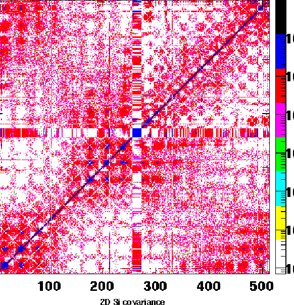
Figure 6.5: Covariance matrix cov($a_i$,$a_j$) of the Si pad array in run 3192. The color scale is logarithmic, units are $MeV^2$. The matrix is symmetric. Increased elements next to the main diagonal indicate the adjacent neighbour cross-talk. Non-uniform overall landscape is due to the beam offset and the beam's geometrical profile. The white diagonals represent the autocorrelation discussed in subsection 6.5.3. The ``cross'' in the middle corresponds to dead channels.

Namely, the channels of the same half-ring (e.g., 1 and 32, 2 and 31, see subsection 6.5.2 for the channel numbering) appear anticorrelated. This is seen on Fig. 6.5 as white diagonal lines. The mechanism is simply the fact that when $i$ and $j$ belong to the same half-ring,

$$a_i = A_i - \frac{1}{16} (A_i + A_j + S_{14}),$$ (78)

where $S_{14}$ is an amplitude sum over 14 other channels of the same half-ring, and

$$a_j = A_j - \frac{1}{16} (A_j + A_i + S_{14}),$$ (79)

then $a_i$ and $a_j$ are anti-correlated no matter what the physical origins of $A_i$ and $A_j$ are. Elimination of this anticorrelation requires subtracting a different term (with $A_i$ and $A_j$ excluded) for every same half-ring pair $(i,j)$, which would complicate the computations enormously. How large is the anticorrelation so induced ? Based on the Eq. 6.25 and 6.26, and using identities C.4 and C.5:

$$(a_i,a_j) = \frac{15^2+1}{16^2} (A_i,A_j) -\frac{15}{16^2}({\mathfrak{D}}[A_i]+{\mathfrak{D}}[A_j])$$

$$-\frac{14}{16^2}( (A_i,S_{14})+ (A_j,S_{14})) + \frac{1}{16^2}{\mathfrak{D}}[S_{14}],$$ (80)

where ${\mathfrak{D}}$ denotes variance. If the leading cause of non-zero cov$(A_i,A_j)$ is the common event multiplicity (which assumption practically amounts to neglecting the identity of the indices $i$ and $j$ as long as $i \neq j$ ), then a crude estimation can be done using

$$(A_i,S_{14}) \approx (A_j,S_{14}) \approx 14 (A_i,A_j),$$ (81)

$${\mathfrak{D}}[S_{14}] \approx 14{\mathfrak{D}}[A_i]+14\times13 (A_i,A_j),$$ (82)

and Eq. 6.27 can be rewritten entirely in terms of a single channel variance ${\mathfrak{D}}[A]$ and a two channel covariance cov$(A_i,A_j)$:

$$(a_i,a_j) = \frac{1}{16}( (A_i,A_j)-{\mathfrak{D}}[A]) \approx -\frac{1}{16}{\mathfrak{D}}[A],$$ (83)

where the last approximation is based on the practical (and expected) observation that $\vert$cov$(A_i,A_j)\vert \ll {\mathfrak{D}}[A]$. The ${\mathfrak{D}}[A]$ can be estimated based on an $RMS^2$ of a histogram like the one shown on Fig. 6.1 (but including all channels) and is approximately $(2.4\times10$keV$)^2 = 0.057 MeV^2$. In other words, we expect to see a number of negative covariance elements around $-0.0036$   MeV$^2$ as one of the features of the matrix.