Kopytine's homepage

Cross-talk evaluation: results and discussion

Now it's time to introduce the measured cross-talk results and discuss their meaning. Figure  6.6 presents the distribution of the covariance matrix elements in magnitude.

Figure 6.6: A distribution of the covariance matrix elements. Run 3192. Information on the cross-talk magnitude is in the distance between the third and fourth peaks (counting from left).

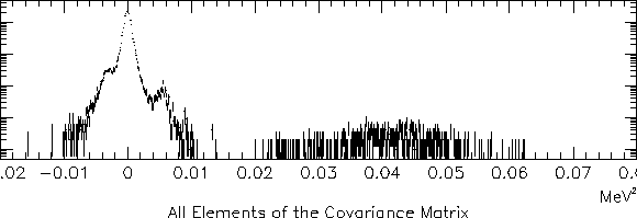Four peaks are clearly seen:

• The largest peak is centered at 0. No cross-talk is therefore the most likely outcome for an arbitrary pair of channels.
• A broad peak is centered between 0.04 and 0.05 MeV$^2$. It contains the diagonal elements of the covariance matrix and does not represent a channel-to-channel influence, but rather a single channel variance, or RMS$^2$ of a distribution like that of Fig. 6.1.
• The peak on the left shoulder of the 0 peak is the one just discussed at length in subsection 6.5.3. It is indeed found where we expect it to be.

  Figure 6.7: A distribution of the covariance matrix elements, that represent correlations between adjacent channels. Run 3192. Same binning as on Fig. 6.6; on that figure, this is seen as the third peak.

  

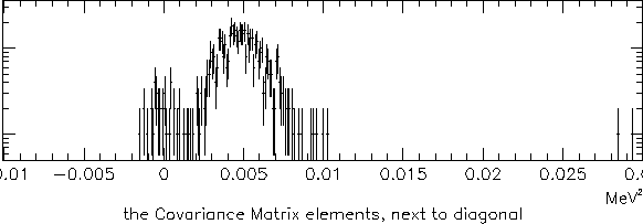• Finally, the peak on the right shoulder of the 0 peak has to be identified with cross-talk. Fig. 6.7 shows this peak separately - it turns out to be the subset of the covariance matrix (i.e. the subset of histogram 6.6) which represents correlations between adjacent channels - namely, the elements next to the main diagonal. As we see, the cross-talk appears as a positive correlation between channels.

What is the magnitude of the cross-talk ? In a typical cross-talk measurement, i.e. by stimulating one channel and registering inductions on the others, at what percentage of the stimulating signal would the induction be ?

To answer this, let's modify equations 6.25 and 6.26 to model the coupling of the two channels with strength $c$:

$$A_i \rightarrow A_i + c A_j,$$

$$A_j \rightarrow A_j + c A_i$$ (84)

and plug in the $A_i$ and $A_j$ so modified in $cov(a_i,a_j)$. What we get (using C.5) is

$$(a_i,a_j)=\frac{15^2+(15c-1)^2}{16^2} -\frac{15(1-15c)}{16^2}({\mathfrak{D}}[A_i] + {\mathfrak{D}}[A_j] )$$

$$-\frac{14+15c}{16^2}( (A_i,S_{14})+ (A_j,S_{14})) + \frac{1}{16^2}{\mathfrak{D}}[S_{14}],$$ (85)

and we repeat the arguments that followed Eq. 6.27. Now we are able to relate $c$ with the observables, because the present analog of Eq. 6.30 reads:

$$(a_i,a_j) \approx \frac{14+30(15c-1)}{16^2} {\mathfrak{D}}[A].$$ (86)

We consider a typical pair of adjacent channels $i$ and $j$, look at Fig. 6.7 and conclude that cov$(a_i,a_j) \approx 0.005 MeV^2$ would be a reasonable estimate; then we recall that ${\mathfrak{D}}[A] \approx 0.057 MeV^2$ (it already figured in the end of subsection 6.5.3). With this input, Eq. 6.33 yields 9% for the effective cross-talk fraction $c$. There are pairs of channels with the coupling parameter $c$ both lower and higher than this.

Why does the cross-talk appear as a positive correlation ? Do not both sources of cross-talk (see subsection 6.5.1) produce an anticorrelation ?

The covariance matrix is an ``integral'' way of looking at the problem. Information so obtained is not sufficient to realistically simulate the effect in the MC detector response program. An event display study indicates that unusual events happen where large positive amplitudes in a couple of neighboring channels are accompanied by noticeable negative amplitudes in the other channels of the same chip (sector), which appear correlated among themselves and anticorrelated with respect to the large amplitude ones.

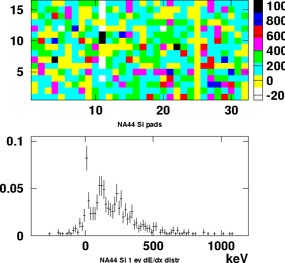
Figure 6.8: An example of a pathological event in the Si pad array. Top panel: the amplitude array. Sector number - horizontal axis, ring number - vertical axis. The $\delta$-free acceptance, used in the analysis, is limited to sectors from 9 through 24. Sector 11 is affected by cross-talk. Sector 25 is dead. Bottom panel: amplitude distribution from this event only. It looks quite normal. The pedestal peak is fine, single and double hit peaks are clearly seen.

Such an example is shown on Fig. 6.8. Sector 11 is affected by cross-talk. There are $16\times(16-1)/2=120$ pairs to be formed among 16 elements (counting only pairs of different elements); in this particular example ( 2 correlated ``positive'' neighbours + 7 correlated ``negatives''), there are 7+7=14 anticorrelated pairs and $7\times(7-1)/2=21$ correlated ones. Therefore, what is, on a large scale, actually an anticorrelation phenomenon, looks from the point of view of a two-point correlation analysis like a correlated one - and sure enough the net contribution of this particular pattern into the covariance matrix will be positive.