Kopytine's homepage

The DWT texture correlation

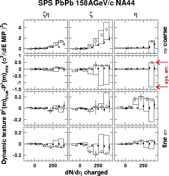
Fig. 7.1 presents a comparison of the DWT dynamic texture in the measured and RQMD-simulated $Pb+Pb$ collision events. The three directional sensitivity modes (diagonal $\zeta \eta$, azimuthal $\zeta$, and pseudorapidity $\eta$) have four scales each, so that there are 12 sets of points in the DWT dynamic texture as a function of the charged multiplicity $\,dN_{ch}/\,d\eta$ bin. The systematic errors on the points (shown by vertical bars) have been evaluated following the procedure described in detail in Section 6.9.

Figure 7.1: Multiplicity dependence of the texture correlation. $\bigcirc$ - the NA44 data, $\bullet$ - RQMD. The boxes show the systematic errors vertically and the boundaries of the multiplicity bins horizontally; the statistical errors are indicated by the vertical bars on the points. The rows correspond to the scale fineness $m$, the columns - to the directional mode $\lambda$ (which can be diagonal $\zeta \eta$, azimuthal $\zeta$, and pseudorapidity $\eta$).

Fig.6.11 demonstrated that the major fraction of the observed texture exists also in mixed events. A detailed account of the causes was discussed in the preceding section (Section 6.9) , including known physics as well as instrumental effects. It is therefore clear that the observable most directly related to the dynamical correlations/fluctuations is not $P^\lambda(m)$ (introduced in 6.6) , but $P^\lambda(m)_{true} - P^\lambda(m)_{mix}$. We find that if one uses the concepts of fluctuation and scale simultaneously, so that scale-local description of fluctuations is possible, then the term ``correlation'' becomes redundant for describing texture, because a ``correlation'' on some scale can always be thought of as a ``fluctuation'' on a larger scale. For example, density of paint on the surface of a chess board looks like a ``correlation without fluctuation'' on the scale of each of its 64 fields, and at the same time, as a ``fluctuation without correlation'' on the scale of the entire chess board. Alternatively, if one uses the term ``correlation'' and specifies scale, then the term ``fluctuation'' becomes redundant.

Figure 7.2: Confidence coefficient as a function of the fluctuation strength. $RMS_{mix}$ denotes $\sqrt{\langle P^\lambda(1)_{mix}^2 - \langle P^\lambda(1)_{mix}\rangle^2\rangle}$. This is the coarsest scale.

This quantity, normalized to the $RMS$ fluctuation of $P^\lambda(m)_{mix}$, can be used to characterize the relative strength of local fluctuations in an event. The distribution for different $\lambda$ (or directions) on the coarsest scale is plotted on Figure 7.2 in an integral way, i.e. as an $\alpha(x)$ graph where for every $x$, $\alpha$ is the fraction of the distribution above $x$.

$$\alpha(x) = {\int_x^{\infty} \frac{\,dN}{\,d\xi} \,d\xi}/ {\int_{-\infty}^{+\infty} \frac{\,dN}{\,d\xi} \,d\xi},$$ (93)

where $\xi$ denotes the fluctuation strength

$$\xi = \frac{P^{\lambda}(1)_{true} - P^{\lambda}(1)_{mix}} {RMS(P^{\lambda}(1)_{mix})},$$ (94)

and $\,dN/\,d\xi$ is the statistical distribution of $\xi$, obtained from the experimentally known distributions of $P^{\lambda}(1)_{true}$ and $P^{\lambda}(1)_{mix}$. Expression 7.2 is constructed to be sensitive to the difference between $P^{\lambda}(1)_{true}$ and $P^{\lambda}(1)_{mix}$, while minimizing detector specifics to enable comparison between different experiments in future. The latter is accomplished by normalizing to $RMS_{mix}$. This normalization also eliminates the trivial multiplicity dependence of the observable.

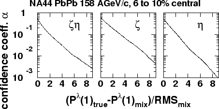
The fluctuation strength observable provides a limit on the frequency and strength of the fluctuations and expresses the result in a model-independent way. The confidence level with which local fluctuations of a given strength (expressed through the EbyE observables via Eq. 7.2) can be excluded is then $1-\alpha$. Fluctuations greater than $3\times RMS_{mix}$ are excluded in the azimuthal and pseudorapidity modes with 90% and 95% confidence, respectively. The monotonic fall of the curve is consistent with the absence of abnormal subsamples in the data.

RQMD events were fed into the GEANT detector response simulation (Section 6.8) and analyzed using the same off-line procedure as used for the experimental data. The detector offset with respect to the beam center of gravity and the beam profile were included in the simulation. In a separate simulation run, the beam profile was identified as the cause of the rise of the azimuthal dynamic texture with the multiplicity on the coarse scale. In our experiment, this purely instrumental effect dominates the azimuthal component of the DWT dynamic texture.

The most apparent conclusion from Fig. 7.1 is that a large fraction of the texture (seen on Fig. 6.11) is not dynamic i.e. not different between true and mixed events. Being monotonic (or absent), the change of the data points with multiplicity does not reveal any evidence of a region of impact parameters/baryochemical potentials with qualitatively different properties, such as those of a critical point neighbourhood. The RQMD comparison confirms that particle production via hadronic multiple scattering, following string decays (without critical phenomena or phase transition) can explain the observed results when detector imperfections are taken into account. More detailed discussion of the implications of these data on various phase transition models will be given in Sections 7.4 and 7.5.