Kopytine's homepage

List of Figures

1. The NA44 spectrometer during the Pb beam running. The T0 and the Si pad array are in the target area and are too small to be seen on this scale. The target area is shown in Fig. 3.2
2. NA44 multiplicity detector complex: a) the lead target, the Si pad array and the T0 scintillators; b) the setup exposed to a simulated RQMD Pb+Pb event.
3. Acceptance area of the NA44 spectrometer in the laboratory rapidity $y$ and transverse momentum $p_T$. Top: in the weak field mode; bottom: in the strong field mode.
4. Means of particle identification in the weak field settings
5. Means of particle identification in the strong field settings
6. Understanding the collimator-related uncertainty in the acceptance-corrected pion $\,dN/\,dy$. The horizontal bars show the extent of the fiducial $p_y$ window used. In this plot, other corrections were fixed at the values they had when the study was undertaken.
7. $\,dN/\,dy$ distributions for negative hadrons: solid and open points - from NA49 measurements [41]; the histogram - from RQMD events of comparable centrality.
8. Determination of the trigger centrality by matching the Si and spectrometer multiplicity data. The multiplicity comparison is done withing the same multiplicity classes based on T0 amplitude, see text.
9. Left: correlation between $\,dN/\,d\eta$ obtained by charged track counting in the spectrometer and fired pad counting in the Si, found to be the best for a particular spectrometer setting. Right: positions of the multiplicity bins of the left plot along the ``diagonalized'' and normalized T0 amplitude.
10. $\chi ^2/NDF$ between actual correlations and the one expected on the basis of acceptance simulation, vs the number of points involved, for three different centralities.
11. Illustration of the Si radiation damage correction algorithm in case of the 4GeV negative low angle setting, 4% centrality sample. From left to right, from top to bottom: SI ADC sum vs number of hits for the left and right parts of the detector in the valid beam run, with the non-interaction cut shown by the solid line; non-interaction cut on T0 signals in the valid beam run ; distribution of the number of Si noise hits in the valid beam run with the non-interaction cut; the ``dirty'' number of charged tracks in the physics run; the ``purified'' number of charged tracks. See text of Subsection  4.2.9
12. Comparison of the average charged track multiplicities measured independently by the left and right sides of the Si detector in the runs with different field sign. See text of Subsection  4.2.10.
13. Track confidence level distribution in the positive strong field, high angle, pion trigger setting. Top: confidence level distribution in $X$. Bottom: confidence level distribution in $Y$.
14. $N(\bar{C2})/N(C2)$ (see text of subsection 4.4.3) as a function of $UCHAD/UCEM$ for the weak field, high angle, positive polarity setting.
15. Correcting for the Cherenkov veto inefficiency in the strong field case, 4% most central events. The number of rejected kaons is evaluated by subtracting the clean pion $m^2$ line shape scaled by a proper multiplier $\Upsilon$. + = all vetoed tracks $\,dN_{lost}/\,dm^2$; $\Diamond$ = ratio of the pure pion line $\,dN_{clean, light}/\,dm^2$ to the ``all vetoed tracks'' distribution, $\circ$ (also in the insert) = $\,dN(K+p)_{lost}/\,dm^2$ obtained as ``all vetoed tracks'' minus $\Upsilon$ - scaled pion line (see Eq.  4.31). The shaded histogram shows the $m^2$ distribution of $K/p$ tracks which were not vetoed.
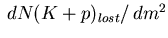
16. Measured transverse kinetic energy distributions of positive and negative kaons for the 4% and 10% most central of Pb+Pb collisions. Two spectrometer angle settings meet at $m_T-m=0.35$ GeV. The fits follow the form $1/m_{T}\,dN/\,dm_{T} \propto exp(-m_{T}/T)$, where $m_{T} = (m^{2}+p_{T}^{2})^{1/2}$. $y$ ranges of the fits are given in Table 2 and are indicated by the horizontal errorbars in the inserts. RQMD predictions for $\vert y-y_{CM}\vert<0.6$ (i.e., within NA44 acceptance) are shown as histograms.
17. Comparison of measured charged kaon and pion yields with RQMD predictions. The vertical error bars indicate statistical and systematic errors, added in quadrature; the horizontal ones - $y$ boundaries of the acceptance used for $p_T$ integration in each spectrometer setting. Open symbols represent spectrometer settings whose $y$ position is shown mirror-reflected around midrapidity (2.92); their solid analogs - the actual settings. RQMD: solid line - standard mode, dashed line - no rescattering.
18. $K/\pi$ ratios in symmetric systems at midrapidity $\vert y-y_{CM}\vert\le \vert y_{proj}-y_{targ}\vert/8$. The solid line shows full solid angle $K/\pi$ in $p+p$ collisions from the interpolation [59]. The data points from other experiments result from an interpolation in $y$ to the midrapidity interval. The E866 data points [60] are also interpolated in the number of participants, for comparison with the SPS data.
19. Comparison of measurements with RQMD predictions: $K^+/\pi ^+$ ratio in the specified rapidity interval around mid-rapidity, as a function of the product of pion and proton $dN/dy$, obtained in the same rapidity interval, in symmetric collisions. $\diamond$ - E866 AuAu, $\bullet$ - NA44 SS, $\circ$ - NA44 PbPb. RQMD: solid line - standard mode, dashed line - no rescattering.
20. A typical calibration fit. Channel 1.
21. Example of a monitoring plot used in the course of the analysis to understand the alignment procedure and the alignment quality. The color (or gray level) corresponds to the pad multiplicity. No misalignment correction is applied. The horizontal lines connect centers of the pads with $\Delta _{i,j}$ sufficiently small for the pairs to be used in formula 6.20 (compare with Fig. 6.3). Run 3192. The $\delta$-contaminated part of the detector is not shown.
22. Another example of a monitoring plot used in the course of the analysis to understand the alignment procedure and the alignment quality. The color (or gray level) corresponds to the pad occupancy. A misalignment correction is applied. One can see how both the acceptances of the pads and their (double differential !) multiplicities are modified. The horizontal lines connect centers of the pads with $\Delta _{i,j}$ sufficiently small for the pairs to be used in formula 6.20 (compare with Fig. 6.2). Run 3192. The $\delta$-contaminated part of the detector is not shown.
23. Alignment results for run 3192. The axes show detector's offsets in $X$ and $Y$ in cm. MIGRAD (see [79]) minimization converged at point $(X,Y) = (0.110 \pm 0.019, 0.031 \pm 0.009)$ cm. The dotted lines cross at the estimated minimum. The contour and the errorbar estimates quoted correspond to the unit deviation of the function from the minimum.
24. Covariance matrix cov($a_i$,$a_j$) of the Si pad array in run 3192. The color scale is logarithmic, units are $MeV^2$. The matrix is symmetric. Increased elements next to the main diagonal indicate the adjacent neighbour cross-talk. Non-uniform overall landscape is due to the beam offset and the beam's geometrical profile. The white diagonals represent the autocorrelation discussed in subsection 6.5.3. The ``cross'' in the middle corresponds to dead channels.
25. A distribution of the covariance matrix elements. Run 3192. Information on the cross-talk magnitude is in the distance between the third and fourth peaks (counting from left).
26. A distribution of the covariance matrix elements, that represent correlations between adjacent channels. Run 3192. Same binning as on Fig. 6.6; on that figure, this is seen as the third peak.
27. An example of a pathological event in the Si pad array. Top panel: the amplitude array. Sector number - horizontal axis, ring number - vertical axis. The $\delta$-free acceptance, used in the analysis, is limited to sectors from 9 through 24. Sector 11 is affected by cross-talk. Sector 25 is dead. Bottom panel: amplitude distribution from this event only. It looks quite normal. The pedestal peak is fine, single and double hit peaks are clearly seen.
28. A distribution of the covariance matrix elements, that represent correlations between adjacent inner channels of sectors. Matrix elements involving dead channels are not shown. Run 3192.
29. Double differential multiplicity distributions of charged particles plotted as a function of azimuthal angle $\zeta$ (with different symbols representing different rings) and of pseudorapidity $\eta$ (with different symbols representing different sectors). The $\zeta$ and $\eta$ are in the aligned coordinates.
30. Power spectra of $7\times 10^3$ events in the multiplicity bin $326<\,dN/\,d\eta<398$. $\bigcirc$ - true events, $\bigtriangleup$ - mixed events, $\Box$ - the average event.
31. Multiplicity dependence of the texture correlation. $\bigcirc$ - the NA44 data, $\bullet$ - RQMD. The boxes show the systematic errors vertically and the boundaries of the multiplicity bins horizontally; the statistical errors are indicated by the vertical bars on the points. The rows correspond to the scale fineness $m$, the columns - to the directional mode $\lambda$ (which can be diagonal $\zeta \eta$, azimuthal $\zeta$, and pseudorapidity $\eta$).
32. Confidence coefficient as a function of the fluctuation strength. $RMS_{mix}$ denotes $\sqrt{\langle P^\lambda(1)_{mix}^2 - \langle P^\lambda(1)_{mix}\rangle^2\rangle}$. This is the coarsest scale.
33. $\,dN/\,dy$ distribution of charged particles in the multifireball event generator in four individual events with different number of fireballs: $\triangle$ - 2 fireballs, $\Box$ - 4 fireballs, $\Diamond$ - 8 fireballs, $\bigcirc$ - 16 fireballs. One can see how the texture becomes smoother as the number of fireballs increases. We remind the reader that the detector's active area covers $2\pi$ azimuthally and pseudorapidity 1.5 to 3.3. In general, acceptance limitations make it more difficult to detect dynamic textures.
34. $\,dN/\,dy$ from negative hadrons obtained in 5% most central events of the multifireball event generator with different clustering parameter $N_{ch}$/fireball.
35. Coarse scale $\eta$ texture correlation in the NA44 data, shown by $\bigcirc$ (from the top right plot of Figure 7.1), is compared with that from the multifireball event generator for three different fireball sizes. Detector response is simulated. The boxes represent systematic errorbars (see caption to Fig. 7.1).